Rosenbrock Function
For a description of the Rosenbrock function minimization problem, see the JupyterLab notebook documentation for this problem.
The python script in this example can be executed from the command line with:
$ python -m yapss.examples.rosenbrock
Functions
YAPSS solution to the minimization of the Rosenbrock function.
Code
"""

YAPSS solution to the minimization of the Rosenbrock function.

"""

__all__ = ["main", "plot_rosenbrock", "setup"]

import numpy as np

# third party imports
from matplotlib import pyplot as plt

# package imports
from yapss import ObjectiveArg, Problem


def setup() -> Problem:
    """Set up the problem to minimize the Rosenbrock problem.

    Returns
    -------
    problem : Problem
        The Rosenbrock function minimization problem.
    """
    # problem has no dynamic phases, and 2 parameters
    problem = Problem(name="Rosenbrock", nx=[], ns=2)

    def objective(arg: ObjectiveArg) -> None:
        """Rosenbrock objective callback function."""
        x0, x1 = arg.parameter
        arg.objective = 100 * (x1 - x0**2) ** 2 + (1 - x0) ** 2

    problem.functions.objective = objective

    # guess
    problem.guess.parameter = -1.2, 1.0

    # yapss options
    problem.derivatives.order = "second"
    problem.derivatives.method = "auto"

    # ipopt options
    problem.ipopt_options.tol = 1e-20
    problem.ipopt_options.print_level = 5

    return problem


def plot_rosenbrock() -> None:
    """Make a contour plot of the Rosenbrock function."""
    x0 = np.linspace(-2, 2, 400)
    x1 = np.linspace(-1, 3, 400)
    x0_grid, x1_grid = np.meshgrid(x0, x1)
    f = 100 * (x1_grid - x0_grid**2) ** 2 + (1 - x0_grid) ** 2

    plt.figure(1)
    levels = [1, 3, 10, 30, 100, 300, 1000, 3000]
    cp = plt.contour(x0, x1, f, levels, colors="black", linewidths=0.5)
    plt.clabel(cp, inline=1, fontsize=8)
    plt.plot(1, 1, ".r", markersize=10)
    plt.xlabel(r"$x_0$")
    plt.ylabel(r"$x_1$")
    plt.title("Rosenbrock function")
    plt.xticks(range(-2, 3))
    plt.yticks(range(-1, 4))
    plt.tight_layout()


def main() -> None:
    """Demonstrate the solution to the Rosenbrock function minimization problem."""
    ocp = setup()
    ocp.derivatives.method = "auto"
    ocp.derivatives.order = "first"
    ocp.ipopt_options.print_level = 5
    solution = ocp.solve()
    x_opt = solution.parameter
    plt.figure()
    print(f"\nThe optimal solution is at the point x = ({x_opt[0]}, {x_opt[1]})")
    plot_rosenbrock()
    plt.show()


if __name__ == "__main__":
    main()
Text Output
******************************************************************************
This program contains Ipopt, a library for large-scale nonlinear optimization.
 Ipopt is released as open source code under the Eclipse Public License (EPL).
         For more information visit https://github.com/coin-or/Ipopt
******************************************************************************

This is Ipopt version 3.14.11, running with linear solver spral.

Number of nonzeros in equality constraint Jacobian...:        0
Number of nonzeros in inequality constraint Jacobian.:        0
Number of nonzeros in Lagrangian Hessian.............:        0

Total number of variables............................:        2
                     variables with only lower bounds:        0
                variables with lower and upper bounds:        0
                     variables with only upper bounds:        0
Total number of equality constraints.................:        0
Total number of inequality constraints...............:        0
        inequality constraints with only lower bounds:        0
   inequality constraints with lower and upper bounds:        0
        inequality constraints with only upper bounds:        0

iter    objective    inf_pr   inf_du lg(mu)  ||d||  lg(rg) alpha_du alpha_pr  ls
   0  2.4200000e+01 0.00e+00 2.16e+02   0.0 0.00e+00    -  0.00e+00 0.00e+00   0
   1  5.1011127e+00 0.00e+00 3.83e+01 -20.3 2.16e+02    -  1.00e+00 9.77e-04f 11
   2  4.1537855e+00 0.00e+00 6.66e+00 -20.3 3.17e-02    -  1.00e+00 1.00e+00f  1
   3  4.1172110e+00 0.00e+00 1.41e+00 -20.3 6.68e-03    -  1.00e+00 1.00e+00f  1
   4  4.1138478e+00 0.00e+00 1.41e+00 -20.3 1.69e-03    -  1.00e+00 1.00e+00f  1
   5  4.1104835e+00 0.00e+00 1.41e+00 -20.3 1.70e-03    -  1.00e+00 1.00e+00f  1
   6  4.1071181e+00 0.00e+00 1.41e+00 -20.3 1.70e-03    -  1.00e+00 1.00e+00f  1
   7  4.0822962e+00 0.00e+00 9.98e+00 -20.3 1.41e+00    -  1.00e+00 3.12e-02f  6
   8  3.8443255e+00 0.00e+00 3.06e+01 -20.3 7.47e-01    -  1.00e+00 1.00e+00f  1
   9  3.6988415e+00 0.00e+00 5.33e+00 -20.3 5.80e-01    -  1.00e+00 1.00e+00f  1
iter    objective    inf_pr   inf_du lg(mu)  ||d||  lg(rg) alpha_du alpha_pr  ls
  10  3.3152088e+00 0.00e+00 2.27e+00 -20.3 1.68e-01    -  1.00e+00 1.00e+00f  1
  11  2.9568858e+00 0.00e+00 7.41e+00 -20.3 1.84e-01    -  1.00e+00 1.00e+00f  1
  12  2.9202278e+00 0.00e+00 1.86e+01 -20.3 4.84e-01    -  1.00e+00 5.00e-01f  2
  13  2.7122136e+00 0.00e+00 9.58e+00 -20.3 1.15e-01    -  1.00e+00 1.00e+00f  1
  14  2.5807322e+00 0.00e+00 7.78e+00 -20.3 3.40e-02    -  1.00e+00 1.00e+00f  1
  15  2.3268760e+00 0.00e+00 1.50e+01 -20.3 3.01e-01    -  1.00e+00 1.00e+00f  1
  16  2.0281526e+00 0.00e+00 2.76e+00 -20.3 1.47e-01    -  1.00e+00 1.00e+00f  1
  17  1.8126691e+00 0.00e+00 3.81e+00 -20.3 8.02e-02    -  1.00e+00 1.00e+00f  1
  18  1.6383532e+00 0.00e+00 8.83e+00 -20.3 5.69e-01    -  1.00e+00 2.50e-01f  3
  19  1.4959030e+00 0.00e+00 4.54e+00 -20.3 2.15e-02    -  1.00e+00 1.00e+00f  1
iter    objective    inf_pr   inf_du lg(mu)  ||d||  lg(rg) alpha_du alpha_pr  ls
  20  1.1803097e+00 0.00e+00 3.26e+00 -20.3 1.28e-01    -  1.00e+00 1.00e+00f  1
  21  1.0292074e+00 0.00e+00 9.27e+00 -20.3 1.72e-01    -  1.00e+00 1.00e+00f  1
  22  7.5166671e-01 0.00e+00 1.80e+00 -20.3 5.58e-02    -  1.00e+00 1.00e+00f  1
  23  6.0644063e-01 0.00e+00 6.82e+00 -20.3 1.67e-01    -  1.00e+00 1.00e+00f  1
  24  5.2258332e-01 0.00e+00 1.45e+00 -20.3 1.91e-02    -  1.00e+00 1.00e+00f  1
  25  4.0323347e-01 0.00e+00 1.65e+00 -20.3 8.96e-02    -  1.00e+00 1.00e+00f  1
  26  3.3584793e-01 0.00e+00 5.09e+00 -20.3 2.18e-01    -  1.00e+00 5.00e-01f  2
  27  2.4948751e-01 0.00e+00 2.19e+00 -20.3 4.75e-02    -  1.00e+00 1.00e+00f  1
  28  1.9589467e-01 0.00e+00 6.24e+00 -20.3 1.41e-01    -  1.00e+00 1.00e+00f  1
  29  1.2414558e-01 0.00e+00 9.25e-01 -20.3 2.76e-02    -  1.00e+00 1.00e+00f  1
iter    objective    inf_pr   inf_du lg(mu)  ||d||  lg(rg) alpha_du alpha_pr  ls
  30  8.0268179e-02 0.00e+00 1.11e+00 -20.3 9.55e-02    -  1.00e+00 1.00e+00f  1
  31  6.5323884e-02 0.00e+00 4.20e+00 -20.3 1.88e-01    -  1.00e+00 5.00e-01f  2
  32  4.4521129e-02 0.00e+00 1.77e+00 -20.3 2.36e-02    -  1.00e+00 1.00e+00f  1
  33  2.0462411e-02 0.00e+00 1.65e+00 -20.3 1.14e-01    -  1.00e+00 1.00e+00f  1
  34  9.0735624e-03 0.00e+00 8.46e-01 -20.3 7.55e-02    -  1.00e+00 1.00e+00f  1
  35  3.6184056e-03 0.00e+00 1.30e+00 -20.3 7.98e-02    -  1.00e+00 1.00e+00f  1
  36  2.7049277e-03 0.00e+00 1.47e+00 -20.3 4.30e-01    -  1.00e+00 6.25e-02f  5
  37  1.6821951e-04 0.00e+00 3.29e-01 -20.3 4.99e-02    -  1.00e+00 1.00e+00f  1
  38  5.1511289e-05 0.00e+00 1.44e-01 -20.3 7.50e-03    -  1.00e+00 1.00e+00f  1
  39  1.4954442e-06 0.00e+00 4.89e-02 -20.3 1.22e-02    -  1.00e+00 1.00e+00f  1
iter    objective    inf_pr   inf_du lg(mu)  ||d||  lg(rg) alpha_du alpha_pr  ls
  40  4.4755734e-07 0.00e+00 2.42e-02 -20.3 4.33e-04    -  1.00e+00 1.00e+00f  1
  41  1.1094519e-10 0.00e+00 2.44e-05 -20.3 5.50e-04    -  1.00e+00 1.00e+00f  1
  42  2.3488989e-13 0.00e+00 5.82e-06 -20.3 2.20e-05    -  1.00e+00 1.00e+00f  1
  43  2.4752797e-14 0.00e+00 6.29e-06 -20.3 9.04e-07    -  1.00e+00 1.00e+00f  1
  44  1.3467623e-14 0.00e+00 2.76e-06 -20.3 4.17e-07    -  1.00e+00 5.00e-01f  2
  45  5.4799074e-18 0.00e+00 3.93e-08 -20.3 1.91e-07    -  1.00e+00 1.00e+00f  1
  46  6.9464343e-21 0.00e+00 2.72e-09 -20.3 4.35e-09    -  1.00e+00 1.00e+00f  1
  47  3.1166059e-23 0.00e+00 2.01e-10 -20.3 9.20e-11    -  1.00e+00 1.00e+00f  1
  48  4.2436960e-24 0.00e+00 1.96e-11 -20.3 1.77e-11    -  1.00e+00 5.00e-01f  2
  49  6.5741400e-26 0.00e+00 7.16e-12 -20.3 4.38e-12    -  1.00e+00 1.00e+00f  1
iter    objective    inf_pr   inf_du lg(mu)  ||d||  lg(rg) alpha_du alpha_pr  ls
  50  5.1615662e-27 0.00e+00 2.76e-12 -20.3 3.27e-13    -  1.00e+00 1.00e+00f  1
  51  1.0374014e-27 0.00e+00 7.64e-13 -20.3 9.32e-14    -  1.00e+00 1.00e+00f  1
  52  4.9747541e-29 0.00e+00 1.21e-13 -20.3 6.48e-14    -  1.00e+00 1.00e+00f  1
  53  6.7053177e-30 0.00e+00 8.62e-14 -20.3 1.56e-14    -  1.00e+00 1.00e+00f  1
  54  5.2385294e-30 0.00e+00 8.77e-14 -20.3 4.21e-15    -  1.00e+00 1.00e+00   0
  55  5.1275959e-30 0.00e+00 8.79e-14 -20.3 2.50e-15    -  1.00e+00 1.00e+00T  0
  56  5.1275959e-30 0.00e+00 8.79e-14 -20.3 8.79e-14    -  1.00e+00 1.16e-10f 34
  57  5.1275959e-30 0.00e+00 8.79e-14 -20.3 8.79e-14    -  1.00e+00 1.16e-10f 34
  58  5.1275959e-30 0.00e+00 8.79e-14 -20.3 8.79e-14    -  1.00e+00 1.16e-10f 34
  59  5.1275959e-30 0.00e+00 8.79e-14 -20.3 8.79e-14    -  1.00e+00 1.16e-10f 34

Number of Iterations....: 59

                                   (scaled)                 (unscaled)
Objective...............:   5.1275958839365767e-30    5.1275958839365767e-30
Dual infeasibility......:   8.7929663550312436e-14    8.7929663550312436e-14
Constraint violation....:   0.0000000000000000e+00    0.0000000000000000e+00
Variable bound violation:   0.0000000000000000e+00    0.0000000000000000e+00
Complementarity.........:   0.0000000000000000e+00    0.0000000000000000e+00
Overall NLP error.......:   8.7929663550312436e-14    8.7929663550312436e-14


Number of objective function evaluations             = 270
Number of objective gradient evaluations             = 60
Number of equality constraint evaluations            = 0
Number of inequality constraint evaluations          = 0
Number of equality constraint Jacobian evaluations   = 0
Number of inequality constraint Jacobian evaluations = 0
Number of Lagrangian Hessian evaluations             = 0
Total seconds in IPOPT (w/o function evaluations)    =      0.055
Total seconds in NLP function evaluations            =      0.031

EXIT: Solved To Acceptable Level.

The optimal solution is at the point x = (1.0000000000000004, 1.000000000000001)
Plots
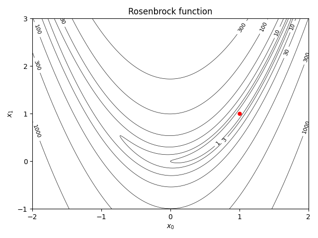
Plotted below is a contour plot of the Rosenbrock function, with the minimum indicated by a red dot. Note that the minimum lies is a long, narrow valley, which makes optimization difficult.