Delta III Launch Vehicle Ascent Problem
For a description of the minimum time to climb problem, see the JupyterLab notebook documentation for this problem.
The python script in this example can be executed from the command line with:
$ python -m yapss.examples.delta_iii_ascent
Functions
YAPSS solution of the Delta III ascent trajectory optimization problem.
- main() None[source]
Demonstrate the solution to the Delta III ascent trajectory optimization problem.
Code
"""
YAPSS solution of the Delta III ascent trajectory optimization problem.
"""
# N803 Argument name should be lowercase
# N806 Variable in function should be lowercase
# ruff: noqa: N803, N806
from __future__ import annotations
__all__ = ["main", "plot_solution", "setup"]
import warnings
# standard library imports
from typing import TYPE_CHECKING, Any
import numpy as np
# third party imports
from matplotlib import pyplot as plt
# package imports
from yapss import ContinuousArg, DiscreteArg, ObjectiveArg, Problem, Solution
from yapss.math import arccos, cos, exp, pi, sin, sqrt
if TYPE_CHECKING:
# package imports
from yapss import Solution
# Suppress only the specific RuntimeWarning message
warnings.filterwarnings(
"ignore",
message="invalid value encountered in divide",
category=RuntimeWarning,
)
# Dynamic Model Parameters
mu = 3.986012e14 # earth gravity parameter
R_e = 6378145.0 # earth radius
g0 = 9.80665 # sea-level gravity
h0 = 7200.0 # atmospheric density scale height
rho0 = 1.225 # sea-level air density
omega_e = 7.29211585e-5 # earth rotation rate
CD = 0.5 # coefficient of drag
S = 4 * pi # aerodynamic reference area
psi_l = 28.5 * pi / 180.0 # latitude of launch site
q_max = 100000.0 # dynamic pressure bound
# Vehicle parameters
# srb, first stage, second stage, payload masses (kg)
pi_s, pi_1, pi_2, pi_p = 19290.0, 104380.0, 19300.0, 4164.0
# propellant masses (kg)
rho_s, rho_1, rho_2 = 17010.0, 95550.0, 16820.0
# dry masses
phi_s = pi_s - rho_s
phi_1 = pi_1 - rho_1
phi_2 = pi_2 - rho_2
# srb, first stage, second stage thrust (N)
Ts, T1, T2 = 628500.0, 1083100.0, 110094.0
# burn times
tau_s, tau_1, tau_2 = 75.2, 261.0, 700.0
# initial total mass of vehicle
m_total = 9 * pi_s + pi_1 + pi_2 + pi_p
# initial time for each phase
t0, t1, t2, t3 = 0.0, 75.2, 150.4, 261.0
# max final time
t4_max = t3 + tau_2
# srb, first stage, second stage specific impulse (sec)
Is = Ts * tau_s / (rho_s * g0)
I1 = T1 * tau_1 / (rho_1 * g0)
I2 = T2 * tau_2 / (rho_2 * g0)
# orbital parameters for desired orbit
a_f, e_f, i_f, Omega_f, omega_f = 24361140, 0.7308, 28.5, 269.8, 130.5
# scaling parameters for IPOPT problem scaling
length_scale = R_e
mu_scale = mu
mass_scale = m_total
velocity_scale = sqrt(mu_scale / length_scale)
time_scale = length_scale / velocity_scale
state_scale = np.ones([7])
state_scale[:3] *= length_scale
state_scale[3:6] *= velocity_scale
state_scale[6] *= mass_scale
# initial position
r0_vec = R_e * cos(psi_l), 0.0, R_e * sin(psi_l)
mi_0 = 9 * pi_s + pi_1 + pi_2 + pi_p
mf_0 = mi_0 - 6 * rho_s - tau_s / tau_1 * rho_1
mi_1 = mf_0 - 6 * phi_s
mf_1 = mi_1 - 3 * rho_s - tau_s / tau_1 * rho_1
mi_2 = mf_1 - 3 * phi_s
mf_2 = mi_2 - (1 - 2 * tau_s / tau_1) * rho_1
mi_3 = mf_2 - phi_1
def cross(x1: Any, x2: Any) -> Any:
"""Vector cross product."""
x3 = [0, 0, 0]
x3[0] = x1[1] * x2[2] - x1[2] * x2[1]
x3[1] = x1[2] * x2[0] - x1[0] * x2[2]
x3[2] = x1[0] * x2[1] - x1[1] * x2[0]
return x3
def mag(x: Any) -> Any:
"""Vector magnitude."""
return (sum(xi**2 for xi in x) + 1e-100) ** 0.5
def dot(x1: Any, x2: Any) -> Any:
"""Vector _dot product."""
return sum(x1[i] * x2[i] for i in range(3))
# noinspection PyPep8Naming
def oe_to_rv( # noqa: PLR0913 (Too many arguments)
a: Any,
e: Any,
i: Any,
Omega: Any,
omega: Any,
nu: Any,
mu_: Any,
) -> Any:
"""Convert orbital elements to cartesian position and velocity.
Parameters
----------
a: semimajor axis
e: eccentricity
i: inclination
Omega: longitude of the ascending node (degrees)
omega: argument of the periapsis (degrees)
nu: true anomaly
mu_: Gravitational parameter
Returns
-------
Tuple[ArrayLike]: Inertial position and velocity vectors
"""
p = a * (1 - e**2)
r = p / (1 + e * cos(nu))
r_vec = np.array([r * cos(nu), r * sin(nu), 0])
v_vec = sqrt(mu_ / p) * np.array([-sin(nu), e + cos(nu), 0])
deg_to_rad = pi / 180
c_O = cos(deg_to_rad * Omega)
s_O = sin(deg_to_rad * Omega)
c_o = cos(deg_to_rad * omega)
s_o = sin(deg_to_rad * omega)
c_i = cos(deg_to_rad * i)
s_i = sin(deg_to_rad * i)
R = np.array(
[
[c_O * c_o - s_O * s_o * c_i, -c_O * s_o - s_O * c_o * c_i, +s_O * s_i],
[s_O * c_o + c_O * s_o * c_i, -s_O * s_o + c_O * c_o * c_i, -c_O * s_i],
[s_o * s_i, c_o * s_i, c_i],
],
)
r_vec = R @ r_vec
v_vec = R @ v_vec
return r_vec, v_vec
def setup() -> Problem:
"""Set up the Delta III ascent optimal control problem.
Returns
-------
Problem
The Delta III ascent optimal control problem.
"""
ocp = Problem(
name="Delta III Ascent Trajectory Optimization",
nx=[7, 7, 7, 7],
nu=[3, 3, 3, 3],
nh=[2, 2, 2, 2],
nd=23,
)
def objective(arg: ObjectiveArg) -> None:
"""Calculate Delta III ascent trajectory optimization problem objective.
The Delta III ascent trajectory optimization problem objective is to maximize the
total mass at the end of the trajectory.
"""
arg.objective = -arg.phase[3].final_state[6]
def continuous(arg: ContinuousArg) -> None:
"""Calculate Delta III ascent trajectory optimization problem dynamics and path constraints.
The constraints are:
* The magnitude of the thrust control vector must be identically one.
* The altitude must always be greater than zero.
"""
for p in arg.phase_list:
state = arg.phase[p].state
r1, r2, r3 = r_vec = state[0:3]
v1, v2, v3 = v_vec = state[3:6]
m = state[6]
u1, u2, u3 = u_vec = arg.phase[p].control
if p == 0:
thrust = 6 * Ts + T1
m_dot = -(6 * Ts / (g0 * Is) + T1 / (g0 * I1))
elif p == 1:
thrust = 3 * Ts + T1
m_dot = -(3 * Ts / (g0 * Is) + T1 / (g0 * I1))
elif p == 2: # noqa: PLR2004
thrust = T1
m_dot = -T1 / (g0 * I1)
elif p == 3: # noqa: PLR2004
thrust = T2
m_dot = -T2 / (g0 * I2)
else:
raise ValueError # pragma: no cover
# kinematics
r1_dot, r2_dot, r3_dot = v1, v2, v3
# air density
r = (r1**2 + r2**2 + r3**2) ** 0.5
h = r - R_e
rho = rho0 * exp(-h / h0)
# aerodynamics
omega_cross_r = cross([0, 0, omega_e], r_vec)
vr_vec = [v_vec[i] - omega_cross_r[i] for i in range(3)]
vr = mag(vr_vec)
q_over_vr = 0.5 * rho * vr
q_factor = q_over_vr * CD * S
d1, d2, d3 = -q_factor * vr_vec[0], -q_factor * vr_vec[1], -q_factor * vr_vec[2]
# dynamics
mu_over_r3 = mu / r**3
thrust_over_m = thrust / m
one_over_m = 1 / m
v1_dot = -mu_over_r3 * r1 + thrust_over_m * u1 + one_over_m * d1
v2_dot = -mu_over_r3 * r2 + thrust_over_m * u2 + one_over_m * d2
v3_dot = -mu_over_r3 * r3 + thrust_over_m * u3 + one_over_m * d3
arg.phase[p].dynamics[:] = r1_dot, r2_dot, r3_dot, v1_dot, v2_dot, v3_dot, m_dot
# path constraints
arg.phase[p].path[:] = mag(u_vec), mag(r_vec)
def discrete(arg: DiscreteArg) -> None:
"""Calculate the Delta III ascent trajectory optimization problem discrete constraints.
The discrete constraints are that:
* The final position and velocity of each phase are the same as the
initial position and velocity at the next phase, if there is one.
* The final position and velocity of the last phase is in the desired
orbit.
"""
phase = arg.phase
arg.discrete[0:6] = phase[0].final_state[0:6] - phase[1].initial_state[0:6]
arg.discrete[6:12] = phase[1].final_state[0:6] - phase[2].initial_state[0:6]
arg.discrete[12:18] = phase[2].final_state[:6] - phase[3].initial_state[:6]
x = phase[3].final_state
r = x[:3]
v = x[3:6]
oe = rv_to_oe(r, v)
arg.discrete[18:23] = oe
ocp.functions.objective = objective
ocp.functions.continuous = continuous
ocp.functions.discrete = discrete
def rv_to_oe(r_vec: Any, v_vec: Any) -> Any:
r"""Compute orbital elements from position and velocity vectors.
The function is a simplified calculation of (some of) the orbital elements, without
checking for special cases.
Parameters
----------
r_vec : 3-dimensional position vector
v_vec : 3-dimensional velocity vector
Returns
-------
Tuple[int]
Five of the six orbital elements: semimajor axis, eccentricity, inclination,
longitude of the ascending node, argument of the periapsis
"""
# http://www.aerospacengineering.net/determining-orbital-elements/
r = mag(r_vec)
v = mag(v_vec)
h_vec = cross(r_vec, v_vec)
h = mag(h_vec)
n_vec = cross([0, 0, 1], h_vec)
n = mag(n_vec)
e0 = ((v**2 - mu / r) * r_vec[0] - dot(r_vec, v_vec) * v_vec[0]) / mu
e1 = ((v**2 - mu / r) * r_vec[1] - dot(r_vec, v_vec) * v_vec[1]) / mu
e2 = ((v**2 - mu / r) * r_vec[2] - dot(r_vec, v_vec) * v_vec[2]) / mu
e_vec = (e0, e1, e2)
e = mag(e_vec)
a = 1 / (2 / r - v**2 / mu)
i = arccos(h_vec[2] / h) * 180 / pi
Omega = 360 - arccos(n_vec[0] / n) * 180 / pi
omega = arccos(dot(n_vec, e_vec) / (n * e)) * 180 / pi
return a, e, i, Omega, omega
x0 = R_e * cos(psi_l), 0.0, R_e * sin(psi_l)
v0 = [0.0, R_e * omega_e * cos(psi_l), 0.0]
state_0 = 7 * [0.0]
state_0[:3] = x0
state_0[3:6] = v0
state_0[6] = mi_0
r_max = 2 * R_e
v_max = 10000.0
# 10 kg leeway on box bounds
ten = 10
# box bounds on position and velocity
for p in range(4):
bounds = ocp.bounds.phase[p]
bounds.initial_state.lower[:6] = 3 * [-r_max] + 3 * [-v_max]
bounds.initial_state.upper[:6] = 3 * [r_max] + 3 * [v_max]
bounds.state.lower[:6] = 3 * [-r_max] + 3 * [-v_max]
bounds.state.upper[:6] = 3 * [r_max] + 3 * [v_max]
bounds.final_state.lower[:6] = 3 * [-r_max] + 3 * [-v_max]
bounds.final_state.upper[:6] = 3 * [r_max] + 3 * [v_max]
# phase 0 time and state bounds
bounds = ocp.bounds.phase[0]
bounds.initial_time.lower = bounds.initial_time.upper = t0
bounds.final_time.lower = bounds.final_time.upper = t1
bounds.initial_state.lower[:] = bounds.initial_state.upper[:] = state_0
bounds.state.lower[6] = mf_0 - ten
bounds.state.upper[6] = mi_0 + ten
bounds.final_state.lower[6] = mf_0 - ten
bounds.final_state.upper[6] = mi_0 + ten
# phase 1
bounds = ocp.bounds.phase[1]
bounds.initial_time.lower = bounds.initial_time.upper = t1
bounds.final_time.lower = bounds.final_time.upper = t2
bounds.initial_state.lower[6] = bounds.initial_state.upper[6] = mi_1
bounds.state.lower[6] = mf_1 - ten
bounds.state.upper[6] = mi_1 + ten
bounds.final_state.lower[6] = mf_1 - ten
bounds.final_state.upper[6] = mi_1 + ten
# phase 2
bounds = ocp.bounds.phase[2]
bounds.initial_time.lower = bounds.initial_time.upper = t2
bounds.final_time.lower = bounds.final_time.upper = t3
bounds.initial_state.lower[6] = bounds.initial_state.upper[6] = mi_2
bounds.state.lower[6] = mf_2 - ten
bounds.state.upper[6] = mi_2 + ten
bounds.final_state.lower[6] = mf_2 - ten
bounds.final_state.upper[6] = mi_2 + ten
# phase 3
bounds = ocp.bounds.phase[3]
bounds.initial_time.lower = bounds.initial_time.upper = t3
bounds.final_time.lower = t3
bounds.final_time.upper = t4_max
bounds.initial_state.lower[6] = bounds.initial_state.upper[6] = mi_3
bounds.state.lower[6] = pi_p - ten
bounds.state.upper[6] = mi_3 + ten
bounds.final_state.lower[6] = pi_p
bounds.final_state.upper[6] = mi_3 + ten
# path and control constraints
for p_ in range(4):
ocp.bounds.phase[p_].path.lower[:] = 1, R_e
ocp.bounds.phase[p_].path.upper[0] = 1
ocp.bounds.phase[p_].control.lower[:] = -1.1
ocp.bounds.phase[p_].control.upper[:] = +1.1
# discrete constraints
ocp.bounds.discrete.lower[:18] = ocp.bounds.discrete.upper[:18] = 0
ocp.bounds.discrete.lower[18:23] = ocp.bounds.discrete.upper[18:23] = (
a_f,
e_f,
i_f,
Omega_f,
omega_f,
)
# time guess
ocp.guess.phase[0].time = (t0, t1)
ocp.guess.phase[1].time = (t1, t2)
ocp.guess.phase[2].time = (t2, t3)
ocp.guess.phase[3].time = (t3, t4_max)
for p in range(4):
ocp.guess.phase[p].state = np.zeros([7, 2])
# mass guess
ocp.guess.phase[0].state[6] = (mi_0, mf_0)
ocp.guess.phase[1].state[6] = (mi_1, mf_1)
ocp.guess.phase[2].state[6] = (mi_2, mf_2)
ocp.guess.phase[3].state[6] = (mi_3, pi_p)
# position, velocity, and control guess
for p_ in range(2):
guess = ocp.guess.phase[p_]
guess.state[:3] = 2 * (x0[0],), 2 * (x0[1],), 2 * (x0[2],)
guess.state[3:6] = 2 * (v0[0],), 2 * (v0[1],), 2 * (v0[2],)
guess.control = [[0.0, 0.0], [1.0, 1.0], [0.0, 0.0]]
# terminal state
temp = np.concatenate(oe_to_rv(a_f, e_f, i_f, Omega_f, omega_f, 0, mu))
temp = np.array([temp, temp]).transpose()
for p_ in range(2, 4):
guess = ocp.guess.phase[p_]
guess.state[:6] = temp
guess.control = [[0.0, 0.0], [1.0, 1.0], [0.0, 0.0]]
ocp.derivatives.method = "auto"
ocp.derivatives.order = "second"
ocp.ipopt_options.max_iter = 1000
ocp.ipopt_options.print_level = 3
# scales
for p in range(4):
ocp.scale.phase[p].state[0:3] = length_scale
ocp.scale.phase[p].state[3:6] = velocity_scale
ocp.scale.phase[p].state[6] = mass_scale
ocp.scale.phase[p].dynamics[0:3] = length_scale
ocp.scale.phase[p].dynamics[3:6] = velocity_scale
ocp.scale.phase[p].dynamics[6] = mass_scale
ocp.scale.phase[p].time = time_scale
ocp.scale.phase[p].path[:] = 1, length_scale
ocp.scale.phase[p].path[1] = length_scale / 2
for p in range(3):
ocp.scale.discrete[0 + 6 * p : 3 + 6 * p] = length_scale
ocp.scale.discrete[3 + 6 * p : 6 + 6 * p] = velocity_scale
ocp.scale.discrete[18] = length_scale
ocp.scale.objective = 8_000
# default mesh configuration is a bit slow for this problem
m, n = 5, 5
for p_ in range(4):
ocp.mesh.phase[p_].collocation_points = m * (n,)
ocp.mesh.phase[p_].fraction = m * (1.0 / m,)
ocp.spectral_method = "lgl"
ocp.ipopt_options.tol = 1e-20
ocp.ipopt_options.constr_viol_tol = 1e-20
ocp.ipopt_options.dual_inf_tol = 1e-20
ocp.ipopt_options.compl_inf_tol = 1e-20
return ocp
def plot_solution(solution: Solution) -> None:
"""Plot the solution.
Parameters
----------
solution : Solution
The solution to the Delta III ascent trajectory optimization problem.
"""
# extract the state, control, costate, dynamics, and time variables
x = [solution.phase[p].state for p in range(4)]
u = [solution.phase[p].control for p in range(4)]
t = [solution.phase[p].time for p in range(4)]
tu = [solution.phase[p].time_c for p in range(4)]
# velocity for plotting
v = 4 * [t]
for phase in range(4):
v[phase] = np.sqrt(x[phase][3] ** 2 + x[phase][4] ** 2 + x[phase][5] ** 2)
# plot settings
color = ("darkblue", "maroon", "darkorange")
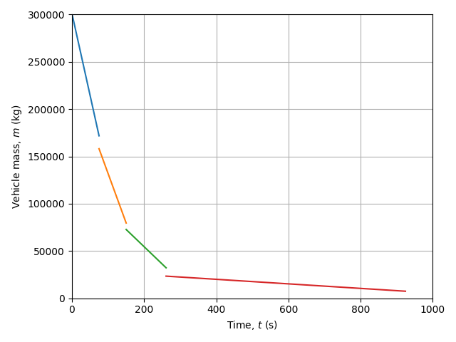
# mass
plt.figure(1)
for p in range(4):
plt.plot(t[p], x[p][6])
plt.ylabel("Vehicle mass, $m$ (kg)")
plt.ylim([0, 300000])
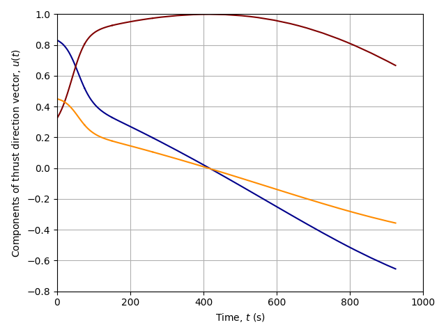
# control vector
plt.figure(2)
for p in range(4):
for i in range(3):
plt.plot(tu[p], u[p][i], color[i])
plt.ylabel("Components of thrust direction vector, $u(t)$")
plt.ylim([-0.8, 1.0])
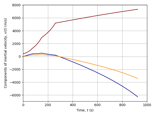
# velocity vector
plt.figure(3)
for phase in range(4):
for i in range(3, 6):
plt.plot(t[phase], x[phase][i] - x[0][i][0] * 0, color[i - 3])
plt.ylabel("Components of inertial velocity, $v(t)$ (m/s)")
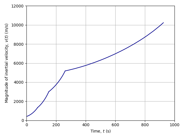
# total velocity
plt.figure(4)
for phase in range(4):
plt.plot(t[phase], v[phase], color[0])
plt.ylabel("Magnitude of inertial velocity, $v(t)$ (m/s)")
plt.ylim([0, 12000])
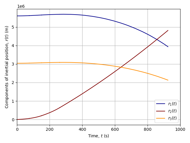
# position vector
plt.figure(5)
for phase in range(4):
for i in range(3):
plt.plot(t[phase], x[phase][i] - x[0][i][0] * 0, color[i])
plt.ylabel("Components of inertial position, $r(t)$ (m)")
plt.legend([r"$r_{1}(t)$", r"$r_{2}(t)$", r"$r_{3}(t)$"])
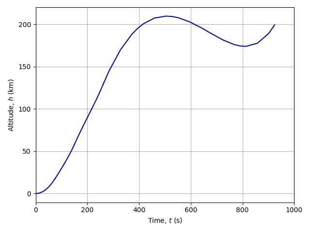
# altitude
plt.figure(6)
plt.clf()
for phase in range(4):
h = np.sqrt(sum(x[phase][i] ** 2 for i in range(3))) - R_e
plt.plot(t[phase], h / 1000, color[0])
plt.ylabel(r"Altitude, $h$ (km)")
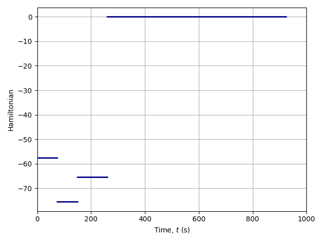
# hamiltonian
plt.figure(7)
plt.clf()
for p in range(4):
plt.plot(tu[p], solution.phase[p].hamiltonian, color[0], linewidth=2)
plt.ylabel(r"Hamiltonian")
# common figure elements
for i in range(1, 8):
plt.figure(i)
plt.xlim([0, 1000])
plt.xlabel("Time, $t$ (s)")
plt.grid(visible=True)
plt.tight_layout()
def main() -> None:
"""Demonstrate the solution to the Delta III ascent trajectory optimization problem."""
problem = setup()
ocp = problem
ocp.ipopt_options.print_level = 3
ocp.derivatives.method = "auto"
ocp.derivatives.order = "second"
ocp.spectral_method = "lgl"
ocp.ipopt_options.linear_solver = "mumps"
ocp.ipopt_options.max_iter = 300
solution = problem.solve()
plot_solution(solution)
plt.show()
if __name__ == "__main__":
main()
Text Output
******************************************************************************
This program contains Ipopt, a library for large-scale nonlinear optimization.
 Ipopt is released as open source code under the Eclipse Public License (EPL).
         For more information visit https://github.com/coin-or/Ipopt
******************************************************************************

Total number of variables............................:      971
                     variables with only lower bounds:        0
                variables with lower and upper bounds:      831
                     variables with only upper bounds:        0
Total number of equality constraints.................:      807
Total number of inequality constraints...............:       88
        inequality constraints with only lower bounds:       88
   inequality constraints with lower and upper bounds:        0
        inequality constraints with only upper bounds:        0


Number of Iterations....: 79

                                   (scaled)                 (unscaled)
Objective...............:  -9.4121403351434119e-01   -7.5297122681147293e+03
Dual infeasibility......:   2.8447533538402862e-13    2.2204465142342694e-13
Constraint violation....:   1.1006090181650260e-14    7.0198439061641693e-08
Variable bound violation:   0.0000000000000000e+00    0.0000000000000000e+00
Complementarity.........:   6.2500000000182493e-25    5.0000000000145992e-21
Overall NLP error.......:   2.8447533538402862e-13    7.0198439061641693e-08


Number of objective function evaluations             = 186
Number of objective gradient evaluations             = 77
Number of equality constraint evaluations            = 186
Number of inequality constraint evaluations          = 186
Number of equality constraint Jacobian evaluations   = 81
Number of inequality constraint Jacobian evaluations = 81
Number of Lagrangian Hessian evaluations             = 79
Total seconds in IPOPT (w/o function evaluations)    =      0.437
Total seconds in NLP function evaluations            =      1.711

EXIT: Solved To Acceptable Level.
Plots
Altitude
Vehicle Position Vector
Total Vehicle Velocity
Vehicle Velocity Vector
Vehicle Mass
Control Inputs
Hamiltonian