Brachistochrone
For a description of the brachistochrone problem with wall constraints as in this script, see the JupyterLab notebook Tutorial Example.
This script provides a detailed implementation of the brachistochrone problem that includes user-defined derivatives. (User-defined derivatives are almost never necessary.) For a script that implements the brachistochrone problem without user-defined derivatives, see the example of a minimal implementation of the brachistochrone.
This example script has user-defined methods for computing the first and second derivatives of the objective and continuous functions. User-defined derivatives can be faster to compute than derivatives computed by automatic differentiation, but not by a large factor. Because for most problems as much time is spent in the Ipopt solver as in derivative functions evaluation, even a substantial speedup in derivative evaluation may not result in a significant speedup in the overall solution time, and so it’s almost never worth the effort to implement user-defined derivatives.
The python script in this example can be executed from the command line with:
$ python -m yapss.examples.brachistochrone
Functions
YAPSS solution to the brachistochrone optimal control problem with user-defined derivatives.
Code
"""
YAPSS solution to the brachistochrone optimal control problem with user-defined derivatives.
"""
__all__ = ["main", "plot_solution", "setup"]
# third party imports
import matplotlib.pyplot as plt
# package imports
from yapss import (
ContinuousArg,
ObjectiveArg,
ObjectiveGradientArg,
ObjectiveHessianArg,
Problem,
Solution,
)
from yapss.math import cos, pi, sin
def setup(*, wall: bool = False) -> Problem:
"""Set up the brachistochrone optimal control problem.
Parameters
----------
wall : bool
Whether to include a wall that bounds the trajectory. Default is False.
Returns
-------
Problem
The brachistochrone optimal control problem.
"""
nh = [1] if wall else [0]
ocp = Problem(name="Brachistochrone", nx=[3], nu=[1], nq=[0], nh=nh)
ocp.auxdata.g0 = 32.174
def objective(arg: ObjectiveArg) -> None:
arg.objective = arg.phase[0].final_time
def objective_gradient(arg: ObjectiveGradientArg) -> None:
arg.gradient[0, "tf", 0] = 1
def objective_hessian(_: ObjectiveHessianArg) -> None:
return
def continuous(arg: ContinuousArg) -> None:
x, y, v = arg.phase[0].state
(u,) = arg.phase[0].control
g0 = arg.auxdata.g0
arg.phase[0].dynamics[:] = v * cos(u), v * sin(u), g0 * sin(u)
if wall:
path = y - x / 2 - 0.1
arg.phase[0].path[:] = (path,)
def continuous_jacobian(arg: ContinuousArg) -> None:
_, _, v = arg.phase[0].state
(u,) = arg.phase[0].control
g0 = arg.auxdata.g0
jacobian = arg.phase[0].jacobian
jacobian[("f", 0), ("x", 2)] = cos(u)
jacobian[("f", 0), ("u", 0)] = -v * sin(u)
jacobian[("f", 1), ("x", 2)] = sin(u)
jacobian[("f", 1), ("u", 0)] = v * cos(u)
jacobian[("f", 2), ("u", 0)] = g0 * cos(u)
if wall:
jacobian[("h", 0), ("x", 0)] = -1 / 2
jacobian[("h", 0), ("x", 1)] = 1
def continuous_hessian(arg: ContinuousArg) -> None:
_, _, v = arg.phase[0].state
(u,) = arg.phase[0].control
g0 = arg.auxdata.g0
hessian = arg.phase[0].hessian
hessian[("f", 0), ("x", 2), ("u", 0)] = -sin(u)
hessian[("f", 0), ("u", 0), ("u", 0)] = -v * cos(u)
hessian[("f", 1), ("x", 2), ("u", 0)] = cos(u)
hessian[("f", 1), ("u", 0), ("u", 0)] = -v * sin(u)
hessian[("f", 2), ("u", 0), ("u", 0)] = -g0 * sin(u)
# functions
ocp.functions.objective = objective
ocp.functions.objective_gradient = objective_gradient
ocp.functions.objective_hessian = objective_hessian
ocp.functions.continuous = continuous
ocp.functions.continuous_jacobian = continuous_jacobian
ocp.functions.continuous_hessian = continuous_hessian
# bounds
bounds = ocp.bounds.phase[0]
bounds.initial_time.lower = bounds.initial_time.upper = 0
bounds.final_time.lower = 0
bounds.initial_state.lower[:] = bounds.initial_state.upper[:] = 0
bounds.final_state.lower[0] = bounds.final_state.upper[0] = 1
bounds.state.lower[:] = 0
bounds.control.lower[:] = 0
bounds.control.upper[:] = pi / 2
if wall:
bounds.path.upper[0] = 0
# guess
phase = ocp.guess.phase[0]
phase.time = (0.0, 1.0)
phase.state = ((0.0, 1.0), (0.0, 1), (0.0, 1.0))
phase.control = ((0, 0.0),)
# mesh
m, n = 20, 10
ocp.mesh.phase[0].collocation_points = m * [n]
ocp.mesh.phase[0].fraction = m * [1 / m]
# solver options
ocp.ipopt_options.tol = 1e-20
ocp.spectral_method = "lgl"
ocp.derivatives.method = "user"
ocp.ipopt_options.print_level = 3
return ocp
def plot_solution(solution: Solution, *, wall: bool = False) -> None:
"""Plot solution for documentation.
Parameters
----------
solution : Solution
Solution to the brachistochrone optimal control problem as produced by YAPSS.
wall : bool, optional
Whether to include a wall that bounds the trajectory. Default is False.
"""
# extract information from solution
time = solution.phase[0].time
time_c = solution.phase[0].time_c
t0 = solution.phase[0].initial_time
tf = solution.phase[0].final_time
state = solution.phase[0].state
control = solution.phase[0].control
costate = solution.phase[0].costate
hamiltonian = solution.phase[0].hamiltonian
lw = 2
x, y, v = state
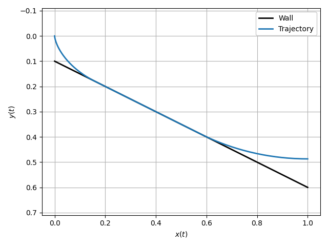
# bead trajectory
plt.figure(1)
plt.clf()
if wall:
plt.plot(x, x / 2 + 0.1, "k", linewidth=lw)
plt.plot(x, y, linewidth=lw)
plt.xlabel("$x(t)$")
plt.ylabel("$y(t)$")
plt.xlim([-0.05, 1.05])
plt.ylim([0.7, -0.05])
plt.axis("equal")
if wall:
plt.legend(("Wall", "Trajectory"), framealpha=1.0)
plt.draw()
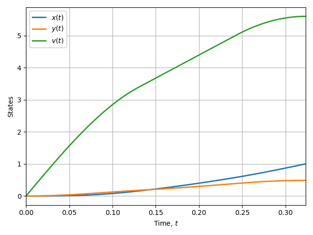
# state vector
plt.figure(2)
plt.clf()
plt.plot(time, x, time, y, time, v, linewidth=lw)
plt.xlabel("Time, $t$")
plt.ylabel("States")
plt.legend(("$x(t)$", "$y(t)$", "$v(t)$"), framealpha=1.0)
plt.xlim([t0, tf])
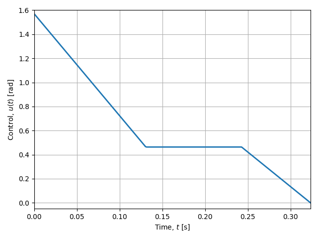
# control
plt.figure(3)
plt.clf()
plt.plot(time_c, control[0], linewidth=lw)
plt.xlabel("Time, $t$ [s]")
plt.ylabel("Control, $u(t)$ [rad]")
plt.ylim([-0.05, 1.6])
plt.xlim([t0, tf])
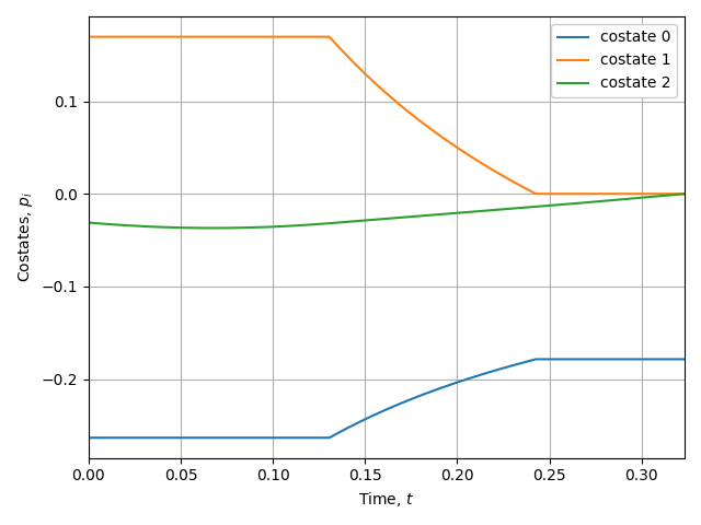
# costates
plt.figure(4)
plt.clf()
plt.plot(time_c, costate[0], time_c, costate[1], time_c, costate[2])
plt.xlim([t0, tf])
plt.xlabel("Time, $t$")
plt.ylabel(r"Costates, $p_{i}$")
plt.legend(["costate 0", "costate 1", "costate 2"], framealpha=1.0)
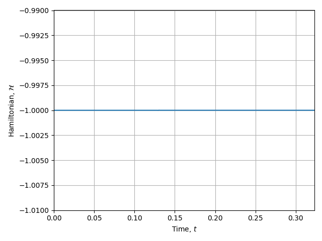
# hamiltonian
plt.figure(5)
plt.clf()
plt.plot(time_c, hamiltonian)
plt.xlim([t0, tf])
plt.ylim([-1.01, -0.99])
plt.xlabel("Time, $t$")
plt.ylabel(r"Hamiltonian, $\mathcal{H}$")
for i in range(1, 6):
plt.figure(i)
plt.tight_layout()
plt.grid()
def main() -> None:
"""Demonstrate the solution to the brachistochrone optimal control problem."""
problem = setup(wall=True)
solution = problem.solve()
plot_solution(solution, wall=True)
plt.show()
if __name__ == "__main__":
main()
Text Output
******************************************************************************
This program contains Ipopt, a library for large-scale nonlinear optimization.
 Ipopt is released as open source code under the Eclipse Public License (EPL).
         For more information visit https://github.com/coin-or/Ipopt
******************************************************************************

Total number of variables............................:      781
                     variables with only lower bounds:      540
                variables with lower and upper bounds:      181
                     variables with only upper bounds:        0
Total number of equality constraints.................:      600
Total number of inequality constraints...............:      182
        inequality constraints with only lower bounds:        1
   inequality constraints with lower and upper bounds:        0
        inequality constraints with only upper bounds:      181


Number of Iterations....: 35

                                   (scaled)                 (unscaled)
Objective...............:   3.2333116383295180e-01    3.2333116383295180e-01
Dual infeasibility......:   1.6653345369377348e-16    1.6653345369377348e-16
Constraint violation....:   9.0716323342121541e-13    9.0716323342121541e-13
Variable bound violation:   0.0000000000000000e+00    0.0000000000000000e+00
Complementarity.........:   9.2950155030469598e-20    9.2950155030469598e-20
Overall NLP error.......:   9.0716323342121541e-13    9.0716323342121541e-13


Number of objective function evaluations             = 36
Number of objective gradient evaluations             = 36
Number of equality constraint evaluations            = 36
Number of inequality constraint evaluations          = 36
Number of equality constraint Jacobian evaluations   = 36
Number of inequality constraint Jacobian evaluations = 36
Number of Lagrangian Hessian evaluations             = 35
Total seconds in IPOPT (w/o function evaluations)    =      0.557
Total seconds in NLP function evaluations            =      0.045

EXIT: Solved To Acceptable Level.
Plots
Optimal Trajectory
State Vector
Control
Costate Vector
Hamiltonian