Minimum Time to Climb Problem

For a description of the minimum time to climb problem, see the JupyterLab notebook documentation for this problem.

The python script in this example can be executed from the command line with:

$ python -m yapss.examples.minimum_time_to_climb

Functions

YAPSS solution of the minimum time to climb problem.

See Arthur E. Bryson Jr., Mukund N. Desai, and William C. Hoffman. Energy-state approximation in performance optimization of supersonic aircraft. Journal of Aircraft, 6(6):481-488, 1969. doi:10.2514/3.44093.

main() → None[source]: Demonstrate the solution of the minimum time to climb problem.

plot_cd0() → None[source]: Plot \(C_{D_0}\) vs. Mach Number \(M\).

plot_density() → None[source]: Plot air density \(\rho\) vs. altitude \(h\).

plot_eta() → None[source]: Plot the induced drag coefficient \(\eta\) vs. Mach number \(M\).

plot_lift_curve_slope() → None[source]: Plot lift curve \(C_{L_\alpha}\) slope vs. Mach number \(M\).

plot_solution(solution: Solution, *, plot_energy_contours: bool = False) → None[source]

Plot the solution to the optimal control problem.

The seven plots are:

Each of the four states (altitude \(h\), velocity \(v\), flight path angle \(\gamma\), and mass \(m\)) vs. time \(t\)
The control variable angle of attack \(\alpha\) vs. time \(t\)
The trajectory of the aircraft, altitude \(h\) vs. velocity \(v\)
The Hamiltonian \(\mathcal{H} = \lambda^T f\) vs. time \(t\)

Parameters:

solutionSolution: The solution to the minimum time to climb optimal control problem.
plot_energy_contoursOptional[bool]: If True, plot contours of constant total energy and excess power.

plot_speed_of_sound() → None[source]: Plot speed of sound \(c\) vs. altitude \(h\).

setup(*, min_fuel: bool = False) → Problem[source]

Set up the Bryson minimum time to climb problem or related minimum fuel to climb problem.

Parameters:

min_fuelbool: True for the minimum fuel to climb problem, False for the minimum time to climb problem.

Returns:

ocpProblem: The minimum time to climb optimal control problem.

Code

"""

YAPSS solution of the minimum time to climb problem.

See Arthur E. Bryson Jr., Mukund N. Desai, and William C. Hoffman. Energy-state approximation
in performance optimization of supersonic aircraft. Journal of Aircraft, 6(6):481-488, 1969.
doi:10.2514/3.44093.

"""

# N806 Variable in function should be lowercase
# ruff: noqa: N806

__all__ = [
    "main",
    "plot_cd0",
    "plot_density",
    "plot_eta",
    "plot_lift_curve_slope",
    "plot_solution",
    "plot_solution",
    "plot_speed_of_sound",
    "setup",
]

# standard library imports
from math import pi

# third party imports
import matplotlib.pyplot as plt
import numpy as np
from numpy.typing import NDArray
from scipy.interpolate import CubicSpline, RBFInterpolator

# package imports
from yapss import ContinuousArg, ObjectiveArg, Problem, Solution

# because we can only use central differences, it's safe to use numpy math
cos = np.cos
sin = np.sin


def objective(arg: ObjectiveArg) -> None:
    """Bryson minimum time to climb objective function.

    Parameters
    ----------
    arg : ObjectiveArg

    Returns
    -------
    None
    """
    if arg.auxdata.min_fuel:
        arg.objective = -arg.phase[0].final_state[3]
    else:
        arg.objective = arg.phase[0].final_time


def continuous(arg: ContinuousArg) -> None:
    """Bryson minimum time to climb continuous dynamics function.

    Parameters
    ----------
    arg : ContinuousArg

    Returns
    -------
    None
    """
    h, v, gamma, mass = arg.phase[0].state
    (alpha,) = arg.phase[0].control

    S = arg.auxdata.S
    g0 = arg.auxdata.g0
    Isp = arg.auxdata.Isp

    rho = get_rho(h)
    c = get_c(h)
    mach = v / c
    CD0 = get_cd0(mach)
    Clalpha = get_cla(mach)
    eta = get_eta(mach)
    thrust = thrust_function(mach, h)
    CD = CD0 + eta * Clalpha * alpha**2
    CL = Clalpha * alpha
    q = 0.5 * rho * v**2
    D = q * S * CD
    L = q * S * CL
    hdot = v * sin(gamma)
    vdot = (thrust * cos(alpha) - D) / mass - g0 * sin(gamma)
    gammadot = (thrust * sin(alpha) + L - mass * g0 * cos(gamma)) / (mass * v)
    mdot = -thrust / (g0 * Isp)
    arg.phase[0].dynamics[:] = hdot, vdot, gammadot, mdot


def setup(*, min_fuel: bool = False) -> Problem:
    """Set up the Bryson minimum time to climb problem or related minimum fuel to climb problem.

    Parameters
    ----------
    min_fuel : bool
        ``True`` for the minimum fuel to climb problem, ``False`` for the
        minimum time to climb problem.

    Returns
    -------
    ocp : Problem
        The minimum time to climb optimal control problem.
    """
    ocp = Problem(name="Bryson Minimum Time to Climb", nx=[4], nu=[1])

    # user functions
    ocp.functions.objective = objective
    ocp.functions.continuous = continuous

    # auxdata
    ocp.auxdata.min_fuel = min_fuel
    ocp.auxdata.S = 530
    ocp.auxdata.g0 = 32.174
    ocp.auxdata.Isp = 1600

    # initial and final conditions
    t0 = 0
    h0, v0, gamma_0, m0 = 0.0, 424.260, 0.0, 42000.0 / ocp.auxdata.g0
    hf, vf, gamma_f = 65600, 968.148, 0.0

    # variable ranges
    tf_min, tf_max = 100, 800
    h_min, h_max = 0, 69000
    v_min, v_max = 1, 2000
    gamma_min = -40 * pi / 180
    gamma_max = 40 * pi / 180
    m_min, m_max = 10, 45000 / ocp.auxdata.g0
    alpha_min, alpha_max = -pi / 4, pi / 4

    # bounds
    bounds = ocp.bounds.phase[0]
    bounds.initial_time.lower = bounds.initial_time.upper = t0
    bounds.final_time.lower = tf_min
    bounds.final_time.upper = tf_max
    bounds.initial_state.lower = bounds.initial_state.upper = h0, v0, gamma_0, m0
    bounds.state.lower = h_min, v_min, gamma_min, m_min
    bounds.state.upper = h_max, v_max, gamma_max, m_max
    bounds.final_state.lower = hf, vf, gamma_f, m_min
    bounds.final_state.upper = hf, vf, gamma_f, m_max
    bounds.control.lower = (alpha_min,)
    bounds.control.upper = (alpha_max,)

    # guess
    guess = ocp.guess.phase[0]
    guess.time = [0, 300]
    guess.state = [[h0, hf], [v0, vf], [gamma_0, gamma_f], [m0, m0]]
    guess.control = [[0, 0]]

    # derivatives -- must use central difference, since tables are not differentiable
    ocp.derivatives.method = "central-difference"

    # scaling
    ocp.scale.phase[0].dynamics = ocp.scale.phase[0].state = 30000.0, 1000.0, 3.0, 500.0
    ocp.scale.phase[0].control[:] = (0.2,)
    ocp.scale.objective = 200
    ocp.scale.phase[0].time = 200

    # solver options
    ocp.ipopt_options.max_iter = 1000
    ocp.derivatives.order = "second"
    ocp.ipopt_options.tol = 1e-8
    ocp.ipopt_options.print_level = 3

    # mesh
    m, n = 15, 15
    ocp.mesh.phase[0].collocation_points = m * (n,)
    ocp.mesh.phase[0].fraction = m * (1.0 / m,)

    return ocp


# mach number array, and altitude array in thousands of feet
mach_data = np.array((0.0, 0.2, 0.4, 0.6, 0.8, 1.0, 1.2, 1.4, 1.6, 1.8))
h_data: NDArray[np.float64] = np.array((0, 5, 10, 15, 20, 25, 30, 40, 50, 70), dtype=float)

# normalize so that each array has range [0,1]
h_data /= 70.0
mach_data /= 1.8

# Thrust data. Note that there are zero entries where the data is unknown or
# undefined. Thrust is in thousands of lbf.
# fmt:off
thrust_data = np.array(
    [[24.2,    0,    0,    0,    0,    0,    0,    0,    0,    0],
     [28.0, 24.6, 21.1, 18.1, 15.2, 12.8, 10.7,    0,    0,    0],
     [28.3, 25.2, 21.9, 18.7, 15.9, 13.4, 11.2,  7.3,  4.4,    0],
     [30.8, 27.2, 23.8, 20.5, 17.3, 14.7, 12.3,  8.1,  4.9,    0],
     [34.5, 30.3, 26.6, 23.2, 19.8, 16.8, 14.1,  9.4,  5.6,  1.1],
     [37.9, 34.3, 30.4, 26.8, 23.3, 19.8, 16.8, 11.2,  6.8,  1.4],
     [36.1, 38.0, 34.9, 31.3, 27.3, 23.6, 20.1, 13.4,  8.3,  1.7],
     [   0, 36.6, 38.5, 36.1, 31.6, 28.1, 24.2, 16.2, 10.0,  2.2],
     [   0,    0,    0, 38.7, 35.7, 32.0, 28.1, 19.3, 11.9,  2.9],
     [   0,    0,    0,    0,    0, 34.6, 31.1, 21.7, 13.3,  3.1]],
)  # fmt:on

# convert to lbf
thrust_data *= 1000

# Find non-empty entries in thrust table, and form argument and value arrays for the
# radial basis function interpolator
thrust_table = []
mh = []
for j, mj in enumerate(mach_data):
    for k, hk in enumerate(h_data):
        thrust_data_point = thrust_data[j][k]
        if thrust_data_point != 0:
            thrust_table.append(thrust_data_point)
            mh.append([mj, hk])

thrust_rbf_interpolator = RBFInterpolator(
    mh,
    thrust_table,
    smoothing=0,
    kernel="cubic",
)


def thrust_function(mach: NDArray[np.float64], h: NDArray[np.float64]) -> NDArray[np.float64]:
    """Determine the thrust available at the given mach numbers and altitudes.

    Parameters
    ----------
    mach : numpy.ndarray
        Array of mach numbers
    h : numpy.ndarray
        Array of altitudes

    Returns
    -------
    numpy.ndarray
        The thrust for each altitude and airspeed pair.
    """
    shape = mach.shape
    length = 1
    for i in shape:
        length *= i
    mach = mach.reshape([length])
    h = h.reshape([length])
    thrust = thrust_rbf_interpolator(np.stack([mach / 1.8, h / 70000], -1))
    return np.array(thrust.reshape(shape), dtype=float)


# make splines of atmospheric data, using the U.S. 1976 Standard Atmosphere in US
# customary units. Data from: http://www.pdas.com/atmosTable1US.html

atmosphere_data = np.array(
    # fmt:off
    #  h     rho       c
    # --  --------  ------
    [[ 0, 2.377E-3, 1116.5],
     [ 5, 2.048E-3, 1097.1],
     [10, 1.756E-3, 1077.4],
     [15, 1.496E-3, 1057.4],
     [20, 1.267E-3, 1036.9],
     [25, 1.066E-3, 1016.1],
     [30, 8.907E-4,  994.8],
     [35, 7.382E-4,  973.1],
     [40, 5.873E-4,  968.1],
     [45, 4.623E-4,  968.1],
     [50, 3.639E-4,  968.1],
     [55, 2.865E-4,  968.1],
     [60, 2.256E-4,  968.1],
     [65, 1.777E-4,  968.1],
     [70, 1.392E-4,  970.9],
     [75, 1.091E-4,  974.3],
     [80, 8.571E-5,  977.6],
     [85, 6.743E-5,  981.0],
     [90, 5.315E-5,  984.3]],
)  # fmt:on

atmosphere_data[:, 0] *= 1000

get_rho = CubicSpline(atmosphere_data[:, 0], atmosphere_data[:, 1])
get_c = CubicSpline(atmosphere_data[:, 0], atmosphere_data[:, 2])

# cubic splines of areodynamic parameters. In order to get desired results, some
# spline points are doubled, effectively forcing the slope at those points to be zero.
# Plots of the resulting spline functions show that the desired result is obtained.
eps = 1e-5

# lift curve slope (CLalpha)
mach_cla = [0, 0.4, 0.8, 0.84 - eps, 0.84, 0.9, 1.0, 1.2, 1.4, 1.6, 1.8]
cla = [3.44, 3.44, 3.44, 3.44, 3.44, 3.58, 4.44, 3.44, 3.01, 2.86, 2.44]
get_cla = CubicSpline(mach_cla, cla)

# baseline drag coefficient (CD0)
mach_cd0 = [0, 0.4, 0.8, 0.86 - eps, 0.86, 0.9, 1.0, 1.2, 1.4, 1.6, 1.8]
cd0 = [0.013, 0.013, 0.013, 0.013, 0.013, 0.014, 0.031, 0.041, 0.039, 0.036, 0.035]
get_cd0 = CubicSpline(mach_cd0, cd0)

# eta
mach_eta = [
    0,
    0.4,
    0.8 - eps,
    0.8,
    0.9,
    1.0,
    1.0 + eps,
    1.2 - eps,
    1.2,
    1.4,
    1.6,
    1.6 + eps,
    1.8 - eps,
    1.8,
]
eta_data = [
    0.54,
    0.54,
    0.54,
    0.54,
    0.75 - 0.01,
    0.79,
    0.79 - eps / 10,
    0.78 + eps / 10,
    0.78,
    0.89,
    0.93,
    0.93,
    0.93,
    0.93,
]
get_eta = CubicSpline(mach_eta, eta_data)

plt.rc("font", family="sans-serif")


def get_excess_power(h: NDArray[np.float64], v: NDArray[np.float64]) -> NDArray[np.float64]:
    """Determine the excess power available to climb at each altitude `h` and airspeed `v`.

    Parameters
    ----------
    h : numpy.ndarray
        Array of altitudes
    v : numpy.ndarray
        Array of velocities

    Returns
    -------
    numpy.ndarray
        The excess power in level flight for each altitude and airspeed
        pair, in level flight.
    """
    # use rough average weight to compute excess power
    g0 = 32.174
    m = 40000 / g0
    S = 530
    rho = get_rho(h)
    c = get_c(h)
    mach = v / c
    CD0 = get_cd0(mach)
    Clalpha = get_cla(mach)
    eta = get_eta(mach)
    qs = 0.5 * rho * v**2 * S
    CL = m * g0 / qs
    alpha = CL / Clalpha
    CD = CD0 + eta * Clalpha * alpha**2
    D = qs * CD
    thrust = thrust_function(mach, h)
    return np.array((thrust - D) * v, dtype=float)


def plot_density() -> None:
    r"""Plot air density :math:`\rho` vs. altitude :math:`h`."""
    h = np.linspace(0.0, 70000.0, 100)
    plt.plot(get_rho(h), h)
    plt.xlabel(r"Density, $\rho$ (slug/ft$^3$)")
    plt.ylabel(r"Altitude, $h$ (ft)")
    plt.xlim([0.0, 0.0025])
    plt.ylim([0.0, 70000.0])
    plt.grid()


def plot_speed_of_sound() -> None:
    """Plot speed of sound :math:`c` vs. altitude :math:`h`."""
    h = np.linspace(0.0, 70000.0, 100)
    plt.plot(get_c(h), h)
    plt.xlabel(r"Speed of sound, $c$ (m/s)")
    plt.ylabel(r"Altitude, $h$ (ft)")
    plt.xlim([960.0, 1120.0])
    plt.ylim([0.0, 70000.0])
    plt.grid()


def plot_lift_curve_slope() -> None:
    r"""Plot lift curve :math:`C_{L_\alpha}` slope vs. Mach number :math:`M`."""
    mach = np.linspace(0, 1.8, 100)
    plt.plot(mach, get_cla(mach))
    plt.plot(mach_cla, cla, ".", markersize=10)
    plt.ylabel(r"Lift curve slope, $C_{L_{\alpha}}$")
    plt.xlabel(r"Mach number, $M$")
    plt.xlim([0.0, 1.8])
    plt.ylim([2, 5])
    plt.grid()


def plot_cd0() -> None:
    """Plot :math:`C_{D_0}` vs. Mach Number :math:`M`."""
    mach = np.linspace(0, 1.8, 100)
    plt.plot(mach, get_cd0(mach))
    plt.plot(mach_cd0, cd0, ".", markersize=10)
    plt.ylabel(r"Baseline drag coefficient, $C_{D_{0}}$")
    plt.xlabel(r"Mach number, $M$")
    plt.xlim([0.0, 1.8])
    plt.ylim([0.01, 0.045])
    plt.grid()


def plot_eta() -> None:
    r"""Plot the induced drag coefficient :math:`\eta` vs. Mach number :math:`M`."""
    mach = np.linspace(0, 1.8, 100)
    plt.plot(mach, get_eta(mach))
    plt.plot(mach_eta, eta_data, ".", markersize=10)
    plt.ylabel(r"Induced drag coefficient, $\eta$")
    plt.xlabel(r"Mach number, $M$")
    plt.xlim([0.0, 1.8])
    plt.ylim([0.5, 0.95])
    plt.grid()


def plot_solution(solution: Solution, *, plot_energy_contours: bool = False) -> None:
    r"""Plot the solution to the optimal control problem.

    The seven plots are:
        * Each of the four states (altitude :math:`h`, velocity :math:`v`, flight
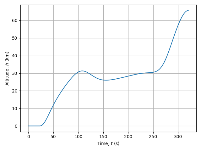
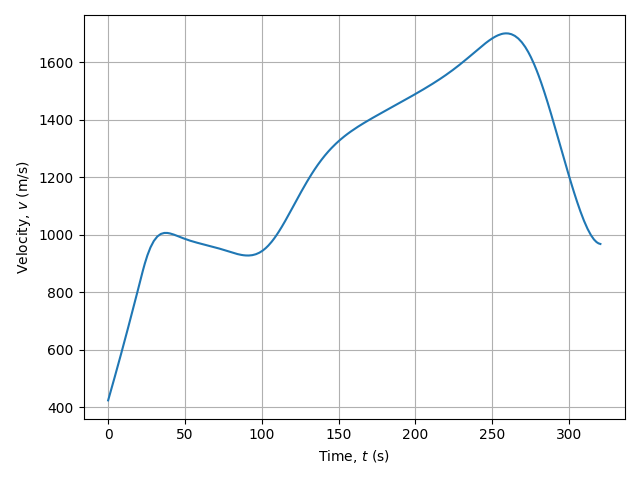
          path angle :math:`\gamma`, and mass :math:`m`) vs. time :math:`t`
        * The control variable angle of attack :math:`\alpha` vs. time :math:`t`
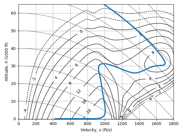
        * The trajectory of the aircraft, altitude :math:`h` vs. velocity :math:`v`
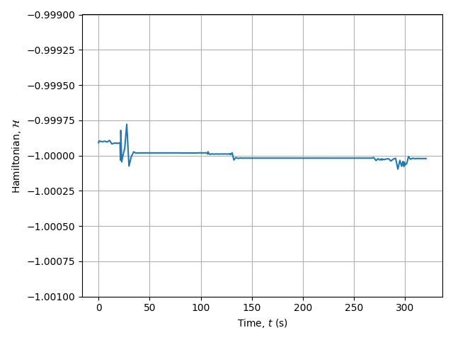
        * The Hamiltonian :math:`\mathcal{H} = \lambda^T f` vs. time :math:`t`

    Parameters
    ----------
    solution : Solution
        The solution to the minimum time to climb optimal control problem.
    plot_energy_contours : Optional[bool]
        If ``True``, plot contours of constant total energy and excess power.
    """
    h, v, gamma, mass = solution.phase[0].state
    t = solution.phase[0].time
    tc = solution.phase[0].time_c
    alpha = solution.phase[0].control[0]
    hamiltonian = solution.phase[0].hamiltonian

    # trajectory
    plt.figure(1)
    # total energy contours
    g0 = 32.174  # 9.80665
    if plot_energy_contours:
        for h_energy in np.linspace(10000, 100000, num=10, endpoint=True):
            h_ = np.linspace(0, h_energy, num=250, endpoint=True)
            v_ = np.sqrt(2 * g0 * (h_energy - h_))
            plt.plot(v_, h_ / 1000, "grey", linewidth=1)

        # excess power contours
        h_grid = np.linspace(-1000, 70000, num=100, dtype=np.float64)
        v_grid = np.linspace(0.1, 1800, num=100, dtype=np.float64)
        v_grid, h_grid = np.meshgrid(v_grid, h_grid)
        power = get_excess_power(h_grid, v_grid)
        cp = plt.contour(
            v_grid,
            h_grid / 1000,
            power / 1e6,
            [-4, -2, 0, 2, 4, 6, 8, 12, 16, 20],
            colors="k",
            linewidths=1,
        )
        plt.clabel(cp, fmt=r"%1.0f")

    plt.plot(v, h / 1000, linewidth=3)
    plt.xlabel(r"Velocity, $v$ (ft/s)")
    plt.ylabel(r"Altitude, $h$ (1000 ft)")
    plt.xlim(0, 1800)
    plt.ylim(-0.3, 65)
    plt.grid()
    plt.tight_layout()

    # altitude
    plt.figure(2)
    plt.plot(t, h / 1000)
    plt.xlabel(r"Time, $t$ (s)")
    plt.ylabel(r"Altitude, $h$ (km)")
    plt.grid()
    plt.tight_layout()

    # velocity
    plt.figure(3)
    plt.plot(t, v)
    plt.xlabel(r"Time, $t$ (s)")
    plt.ylabel(r"Velocity, $v$ (m/s)")
    plt.grid()
    plt.tight_layout()

    # flight path angle
    plt.figure(4)
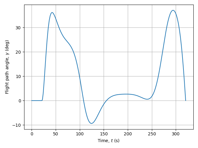
    plt.plot(t, gamma * 180 / np.pi)
    plt.xlabel(r"Time, $t$ (s)")
    plt.ylabel(r"Flight path angle, $\gamma$ (deg)")
    plt.grid()
    plt.tight_layout()

    # mass
    plt.figure(5)
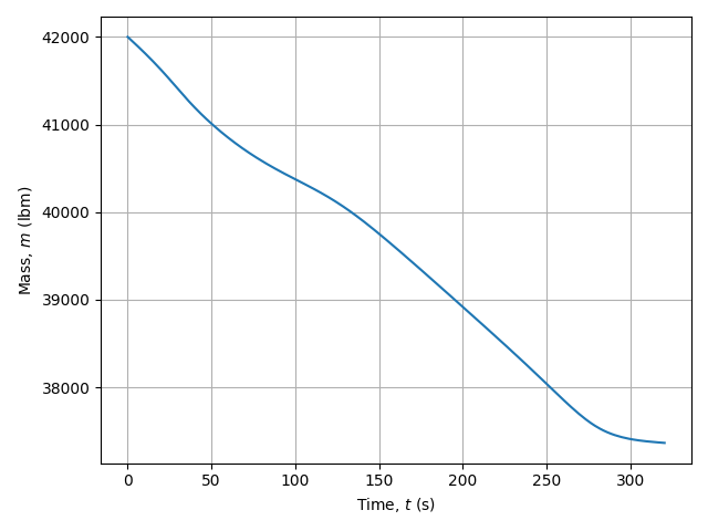
    plt.plot(t, mass * 32.174)
    plt.xlabel(r"Time, $t$ (s)")
    plt.ylabel(r"Mass, $m$ (lbm)")
    plt.grid()
    plt.tight_layout()

    # angle of attack
    plt.figure(6)
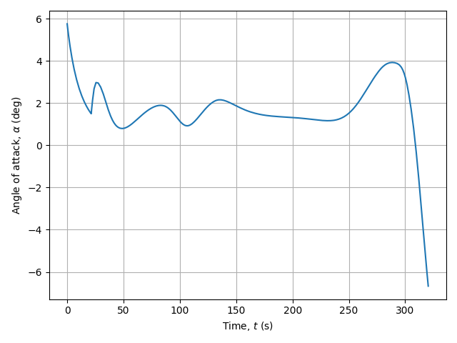
    plt.plot(tc, alpha * 180 / np.pi)
    plt.xlabel(r"Time, $t$ (s)")
    plt.ylabel(r"Angle of attack, $\alpha$ (deg)")
    plt.grid()
    plt.tight_layout()

    # figure 7: Hamiltonian
    plt.figure(7)
    plt.figure(7)
    plt.plot(tc, hamiltonian)
    plt.ylim(-1.001, -0.999)
    plt.xlabel(r"Time, $t$ (s)")
    plt.ylabel(r"Hamiltonian, $\mathcal{H}$")
    plt.grid()
    plt.tight_layout()


def main() -> None:
    """Demonstrate the solution of the minimum time to climb problem."""
    problem = setup()
    solution = problem.solve()
    plot_solution(solution, plot_energy_contours=True)
    plt.show()


if __name__ == "__main__":
    main()

Text Output

******************************************************************************
This program contains Ipopt, a library for large-scale nonlinear optimization.
 Ipopt is released as open source code under the Eclipse Public License (EPL).
         For more information visit https://github.com/coin-or/Ipopt
******************************************************************************

Total number of variables............................:     1109
                     variables with only lower bounds:        0
                variables with lower and upper bounds:     1049
                     variables with only upper bounds:        0
Total number of equality constraints.................:      900
Total number of inequality constraints...............:        1
        inequality constraints with only lower bounds:        1
   inequality constraints with lower and upper bounds:        0
        inequality constraints with only upper bounds:        0


Number of Iterations....: 24

                                   (scaled)                 (unscaled)
Objective...............:   1.6022938034016094e+00    3.2045876068032186e+02
Dual infeasibility......:   4.1771927406053216e-10    1.8656541916194012e-09
Constraint violation....:   2.1415007722680457e-09    2.1415007722680457e-06
Variable bound violation:   0.0000000000000000e+00    0.0000000000000000e+00
Complementarity.........:   1.1422025943058876e-11    2.2844051886117753e-09
Overall NLP error.......:   2.1415007722680457e-09    2.1415007722680457e-06


Number of objective function evaluations             = 25
Number of objective gradient evaluations             = 25
Number of equality constraint evaluations            = 25
Number of inequality constraint evaluations          = 25
Number of equality constraint Jacobian evaluations   = 25
Number of inequality constraint Jacobian evaluations = 25
Number of Lagrangian Hessian evaluations             = 24
Total seconds in IPOPT (w/o function evaluations)    =      0.979
Total seconds in NLP function evaluations            =      0.919

EXIT: Optimal Solution Found.

Plots

Optimal Trajectory

Also shown are contours of energy height (kinetic plus potential energy, divided by mass), and excess power (power available minus power required for level flight).

../_images/minimum_time_to_climb_plot_1.png

Altitude

../_images/minimum_time_to_climb_plot_2.png

Velocity

../_images/minimum_time_to_climb_plot_3.png

Flight Path Angle

../_images/minimum_time_to_climb_plot_4.png

Mass

../_images/minimum_time_to_climb_plot_5.png

Angle of Attack

../_images/minimum_time_to_climb_plot_6.png

Hamiltonian

../_images/minimum_time_to_climb_plot_7.png