Newton’s Minimal Resistance Problem
For a description of Newton’s minimal resistance problem, see the JupyterLab notebook documentation for this problem.
This example script has user-defined methods for computing the first and second derivatives of the objective and continuous functions. User-defined derivatives can be faster to compute than derivatives computed by automatic differentiation, but not by a large factor. Because for most problems as much time is spent in the Ipopt solver as in derivative functions evaluation, even a substantial speedup in derivative evaluation may not result in a significant speedup in the overall solution time, and so it’s almost never worth the effort to implement user-defined derivatives.
The python script in this example can be executed from the command line with:
$ python -m yapss.examples.newton
Functions
YAPSS solution of Newton’s minimal resistance problem.
- plot_solution(solution: Solution) None[source]
Plot the solution to Newton’s minimal resistance problem.
- Parameters:
- solutionSolution
The solution to the Newton’s minimal resistance problem.
- setup(y_max: float = 1.0) Problem[source]
Set up Newton’s minimal resistance problem as an optimal control problem.
- Parameters:
- y_maxfloat, optional
Maximum height of the nosecone, by default 1.0.
- Returns:
- Problem
Newton’s minimal resistance problem as an optimal control problem.
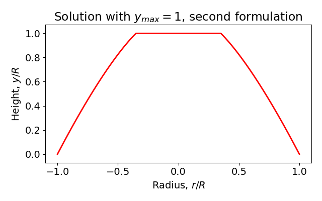
- setup2(y_max: float = 1.0) Problem[source]
Set up alternate formulation of Newton’s minimal resistance problem.
In this alternate formulation, the radius of the flat portion of the nosecone is a parameter to be optimized, and the curve to be optimized starts at this radius. This formulation improves the solution considerably.
- Parameters:
- y_maxfloat, optional
Maximum height of the nosecone, by default 1.0.
- Returns:
- Problem
Newton’s minimal resistance problem as an optimal control problem.
Code
"""
YAPSS solution of Newton's minimal resistance problem.
"""
__all__ = ["main", "plot_solution", "setup", "setup2"]
# third party imports
import matplotlib.pyplot as plt
# package imports
import numpy as np
from yapss import (
ContinuousArg,
ContinuousHessianArg,
ContinuousJacobianArg,
ObjectiveArg,
ObjectiveGradientArg,
ObjectiveHessianArg,
Problem,
Solution,
)
def objective(arg: ObjectiveArg) -> None:
"""Objective function for Newton's minimal resistance problem."""
arg.objective = arg.phase[0].integral[0]
def continuous(arg: ContinuousArg) -> None:
"""Newton's minimal resistance problem dynamics and cost integrand."""
_, yp = arg.phase[0].state
(u,) = arg.phase[0].control
r = arg.phase[0].time
arg.phase[0].dynamics[:] = yp, u
arg.phase[0].integrand[:] = (8 * r / (1 + yp**2),)
# Gradient, Jacobian, and Hessian functions are not required except when
# derivatives.method = "user" option is selected.
def objective_gradient(arg: ObjectiveGradientArg) -> None:
"""Calculate gradient of the objective function for Newton's minimal resistance problem.
Needed only if the ``derivatives.method = "user"`` option is selected.
"""
arg.gradient[0, "q", 0] = 1
def objective_hessian(_: ObjectiveHessianArg) -> None:
"""Calculate Hessian of the objective function for Newton's minimal resistance problem.
Needed only if the ``derivatives.method = "user"`` option is selected.
"""
def continuous_jacobian(arg: ContinuousJacobianArg) -> None:
"""Calculate Jacobian of the dynamics and cost integrand for minimal resistance problem.
Needed only if the ``derivatives.method = "user"`` option is selected.
"""
_, yp = arg.phase[0].state
r = arg.phase[0].time
jacobian = arg.phase[0].jacobian
jacobian[("f", 0), ("x", 1)] = 1
jacobian[("f", 1), ("u", 0)] = 1
jacobian[("g", 0), ("t", 0)] = 8 / (1 + yp**2)
jacobian[("g", 0), ("x", 1)] = -16 * yp * r / (1 + yp**2) ** 2
def continuous_hessian(arg: ContinuousHessianArg) -> None:
"""Calculate Hessian of the dynamics and cost integrand for Newton's minimal resistance problem.
Needed only if the ``derivatives.method = "user"`` option is selected.
"""
_, yp = arg.phase[0].state
r = arg.phase[0].time
hessian = arg.phase[0].hessian
hessian[("g", 0), ("x", 1), ("x", 1)] = 16 * r * (3 * yp**2 - 1) / (1 + yp**2) ** 3
hessian[("g", 0), ("x", 1), ("t", 0)] = -16 * yp / (1 + yp**2) ** 2
# end derivative functions
def setup(y_max: float = 1.0) -> Problem:
"""Set up Newton's minimal resistance problem as an optimal control problem.
Parameters
----------
y_max : float, optional
Maximum height of the nosecone, by default 1.0.
Returns
-------
Problem
Newton's minimal resistance problem as an optimal control problem.
"""
ocp = Problem(
name="Newton's minimal resistance problem",
nx=[2],
nu=[1],
nq=[1],
)
# functions
ocp.functions.objective = objective
ocp.functions.objective_gradient = objective_gradient
ocp.functions.objective_hessian = objective_hessian
ocp.functions.continuous = continuous
ocp.functions.continuous_jacobian = continuous_jacobian
ocp.functions.continuous_hessian = continuous_hessian
# bounds
bounds = ocp.bounds.phase[0]
bounds.initial_time.lower = bounds.initial_time.upper = 0.0
bounds.final_time.lower = bounds.final_time.upper = 1.0
bounds.state.lower[0] = 0
bounds.state.upper = y_max, 0
bounds.control.upper = (0,)
# guess
phase = ocp.guess.phase[0]
phase.time = [0.0, 1.0]
phase.state = [[y_max, 0.0], [-y_max, -y_max]]
phase.control = [[0.0, 0.0]]
# solver settings
ocp.derivatives.order = "second"
# we use the "user" option to demonstrate how to provide derivatives
ocp.derivatives.method = "user"
# ipopt options
ocp.ipopt_options.print_level = 3
return ocp
def objective2(arg: ObjectiveArg) -> None:
"""Improved objective function for Newton's minimal resistance problem."""
arg.objective = arg.phase[0].integral[0] + 4 * arg.phase[0].initial_time ** 2
def objective_gradient2(arg: ObjectiveGradientArg) -> None:
"""Calculate gradient of improved objective function for Newton's minimal resistance problem.
Needed only if the derivatives.method = "user" option is selected.
"""
arg.gradient[0, "q", 0] = 1
arg.gradient[0, "t0", 0] = 8 * arg.phase[0].initial_time
def objective_hessian2(arg: ObjectiveHessianArg) -> None:
"""Calculate Hessian of improved objective function for Newton's minimal resistance problem.
Needed only if the derivatives.method = "user" option is selected.
"""
arg.hessian[(0, "t0", 0), (0, "t0", 0)] = 8
def setup2(y_max: float = 1.0) -> Problem:
"""Set up alternate formulation of Newton's minimal resistance problem.
In this alternate formulation, the radius of the flat portion of the nosecone is a
parameter to be optimized, and the curve to be optimized starts at this radius. This
formulation improves the solution considerably.
Parameters
----------
y_max : float, optional
Maximum height of the nosecone, by default 1.0.
Returns
-------
Problem
Newton's minimal resistance problem as an optimal control problem.
"""
ocp = setup(y_max)
ocp.functions.objective = objective2
ocp.functions.objective_gradient = objective_gradient2
ocp.functions.objective_hessian = objective_hessian2
ocp.bounds.phase[0].initial_time.upper = 0.7
return ocp
def plot_solution(solution: Solution) -> None:
"""Plot the solution to Newton's minimal resistance problem.
Parameters
----------
solution : Solution
The solution to the Newton's minimal resistance problem.
"""
# plot style information
linewidth = 2
plt.rc("font", size=14)
plt.rc("font", family="sans-serif")
# extract information from solution
r = solution.phase[0].time
y, _ = solution.phase[0].state
r = np.concatenate((-r[-1::-1], r))
y = np.concatenate((y[-1::-1], y))
# plot
plt.plot(r, y, "r", linewidth=linewidth)
plt.axis("equal")
plt.xlim([-1, 1])
plt.ylim([-0.1, 2.1])
plt.xlabel("Radius, $r/R$")
plt.ylabel("Height, $y/R$")
plt.tight_layout()
def _truncate_float(number: float, decimals: int = 5) -> float:
"""Truncate a float to a specified number of decimal places."""
factor = 10**decimals
return float(int(number * factor) / factor)
def main() -> None:
"""Demonstrate the solution to Newton's minimal resistance problem."""
# solve problem using the first formulation
problem = setup(y_max=1)
solution1a = problem.solve()
plt.figure(1, figsize=(6.4, 4))
plot_solution(solution1a)
plt.axis((-1.2, 1.2, -0.1, 1.1))
plt.axis("equal")
plt.title("Solution with $y_{max} = 1$, first formulation")
plt.xticks(np.linspace(-1, 1, 5))
plt.tight_layout()
# solve problem using the second formulation
problem = setup2(y_max=1)
solution1b = problem.solve()
plt.figure(2, figsize=(6.4, 4))
plot_solution(solution1b)
plt.axis((-1.2, 1.2, -0.1, 1.1))
plt.axis("equal")
plt.title("Solution with $y_{max} = 1$, second formulation")
plt.xticks(np.linspace(-1, 1, 5))
plt.tight_layout()
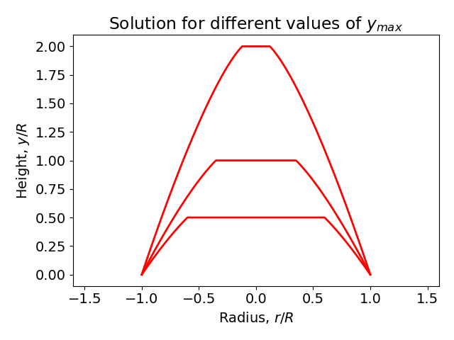
# solve problem for different values of y_max
plt.figure(3)
objective_list: list[float] = []
y_max_list = [0.5, 1, 2]
for y_max in y_max_list:
problem = setup2(y_max=y_max)
solution = problem.solve()
objective_list.append(solution.objective)
plot_solution(solution)
plt.title("Solution for different values of $y_{max}$")
plt.tight_layout()
# print objective values for different values of y_max, in a table
print("\nObjective values for different values of y_max:\n")
print("y_max | Objective (C_D)")
print("------+----------------")
for y_max, objective_value in zip(y_max_list, objective_list):
print(f"{y_max:5.2f} | {_truncate_float(objective_value):8.5f}...")
plt.show()
if __name__ == "__main__":
main()
Text Output
******************************************************************************
This program contains Ipopt, a library for large-scale nonlinear optimization.
 Ipopt is released as open source code under the Eclipse Public License (EPL).
         For more information visit https://github.com/coin-or/Ipopt
******************************************************************************

Total number of variables............................:      294
                     variables with only lower bounds:        0
                variables with lower and upper bounds:       91
                     variables with only upper bounds:      182
Total number of equality constraints.................:      201
Total number of inequality constraints...............:        1
        inequality constraints with only lower bounds:        1
   inequality constraints with lower and upper bounds:        0
        inequality constraints with only upper bounds:        0


Number of Iterations....: 59

                                   (scaled)                 (unscaled)
Objective...............:   1.5033522844316036e+00    1.5033522844316036e+00
Dual infeasibility......:   3.0935965659845183e-09    3.0935965659845183e-09
Constraint violation....:   2.2644555119910592e-09    2.2644555119910592e-09
Variable bound violation:   9.0877317203984134e-09    9.0877317203984134e-09
Complementarity.........:   5.2160175348069363e-09    5.2160175348069363e-09
Overall NLP error.......:   5.2160175348069363e-09    5.2160175348069363e-09


Number of objective function evaluations             = 60
Number of objective gradient evaluations             = 60
Number of equality constraint evaluations            = 60
Number of inequality constraint evaluations          = 60
Number of equality constraint Jacobian evaluations   = 60
Number of inequality constraint Jacobian evaluations = 60
Number of Lagrangian Hessian evaluations             = 59
Total seconds in IPOPT (w/o function evaluations)    =      0.298
Total seconds in NLP function evaluations            =      0.042

EXIT: Optimal Solution Found.
Total number of variables............................:      295
                     variables with only lower bounds:        0
                variables with lower and upper bounds:       92
                     variables with only upper bounds:      182
Total number of equality constraints.................:      201
Total number of inequality constraints...............:        1
        inequality constraints with only lower bounds:        1
   inequality constraints with lower and upper bounds:        0
        inequality constraints with only upper bounds:        0


Number of Iterations....: 16

                                   (scaled)                 (unscaled)
Objective...............:   1.4992639218536086e+00    1.4992639218536086e+00
Dual infeasibility......:   3.4050137239924398e-09    3.4050137239924398e-09
Constraint violation....:   1.2504534074864182e-09    1.2504534074864182e-09
Variable bound violation:   9.9783786942670577e-09    9.9783786942670577e-09
Complementarity.........:   9.8090854271441426e-10    9.8090854271441426e-10
Overall NLP error.......:   3.4050137239924398e-09    3.4050137239924398e-09


Number of objective function evaluations             = 18
Number of objective gradient evaluations             = 17
Number of equality constraint evaluations            = 18
Number of inequality constraint evaluations          = 18
Number of equality constraint Jacobian evaluations   = 17
Number of inequality constraint Jacobian evaluations = 17
Number of Lagrangian Hessian evaluations             = 16
Total seconds in IPOPT (w/o function evaluations)    =      0.046
Total seconds in NLP function evaluations            =      0.010

EXIT: Optimal Solution Found.
Total number of variables............................:      295
                     variables with only lower bounds:        0
                variables with lower and upper bounds:       92
                     variables with only upper bounds:      182
Total number of equality constraints.................:      201
Total number of inequality constraints...............:        1
        inequality constraints with only lower bounds:        1
   inequality constraints with lower and upper bounds:        0
        inequality constraints with only upper bounds:        0


Number of Iterations....: 26

                                   (scaled)                 (unscaled)
Objective...............:   2.4300290388786467e+00    2.4300290388786467e+00
Dual infeasibility......:   3.1807670707070760e-09    3.1807670707070760e-09
Constraint violation....:   6.2818239499051742e-10    6.2818239499051742e-10
Variable bound violation:   9.9932551123060875e-09    9.9932551123060875e-09
Complementarity.........:   3.4046248623079831e-10    3.4046248623079831e-10
Overall NLP error.......:   3.1807670707070760e-09    3.1807670707070760e-09


Number of objective function evaluations             = 28
Number of objective gradient evaluations             = 27
Number of equality constraint evaluations            = 28
Number of inequality constraint evaluations          = 28
Number of equality constraint Jacobian evaluations   = 27
Number of inequality constraint Jacobian evaluations = 27
Number of Lagrangian Hessian evaluations             = 26
Total seconds in IPOPT (w/o function evaluations)    =      0.069
Total seconds in NLP function evaluations            =      0.017

EXIT: Optimal Solution Found.
Total number of variables............................:      295
                     variables with only lower bounds:        0
                variables with lower and upper bounds:       92
                     variables with only upper bounds:      182
Total number of equality constraints.................:      201
Total number of inequality constraints...............:        1
        inequality constraints with only lower bounds:        1
   inequality constraints with lower and upper bounds:        0
        inequality constraints with only upper bounds:        0


Number of Iterations....: 16

                                   (scaled)                 (unscaled)
Objective...............:   1.4992639218536086e+00    1.4992639218536086e+00
Dual infeasibility......:   3.4050137239924398e-09    3.4050137239924398e-09
Constraint violation....:   1.2504534074864182e-09    1.2504534074864182e-09
Variable bound violation:   9.9783786942670577e-09    9.9783786942670577e-09
Complementarity.........:   9.8090854271441426e-10    9.8090854271441426e-10
Overall NLP error.......:   3.4050137239924398e-09    3.4050137239924398e-09


Number of objective function evaluations             = 18
Number of objective gradient evaluations             = 17
Number of equality constraint evaluations            = 18
Number of inequality constraint evaluations          = 18
Number of equality constraint Jacobian evaluations   = 17
Number of inequality constraint Jacobian evaluations = 17
Number of Lagrangian Hessian evaluations             = 16
Total seconds in IPOPT (w/o function evaluations)    =      0.043
Total seconds in NLP function evaluations            =      0.010

EXIT: Optimal Solution Found.
Total number of variables............................:      295
                     variables with only lower bounds:        0
                variables with lower and upper bounds:       92
                     variables with only upper bounds:      182
Total number of equality constraints.................:      201
Total number of inequality constraints...............:        1
        inequality constraints with only lower bounds:        1
   inequality constraints with lower and upper bounds:        0
        inequality constraints with only upper bounds:        0


Number of Iterations....: 16

                                   (scaled)                 (unscaled)
Objective...............:   6.4170199377206250e-01    6.4170199377206250e-01
Dual infeasibility......:   5.2812526958960995e-09    5.2812526958960995e-09
Constraint violation....:   1.9560146835573278e-09    1.9560146835573278e-09
Variable bound violation:   1.9861985833813378e-08    1.9861985833813378e-08
Complementarity.........:   2.5091521318952312e-09    2.5091521318952312e-09
Overall NLP error.......:   5.2812526958960995e-09    5.2812526958960995e-09


Number of objective function evaluations             = 17
Number of objective gradient evaluations             = 17
Number of equality constraint evaluations            = 17
Number of inequality constraint evaluations          = 17
Number of equality constraint Jacobian evaluations   = 17
Number of inequality constraint Jacobian evaluations = 17
Number of Lagrangian Hessian evaluations             = 16
Total seconds in IPOPT (w/o function evaluations)    =      0.043
Total seconds in NLP function evaluations            =      0.010

EXIT: Optimal Solution Found.

Objective values for different values of y_max:

y_max | Objective (C_D)
------+----------------
 0.50 |   2.43002...
 1.00 |   1.49926...
 2.00 |   0.64170...
Plots
Nosecone Shape for First Formulation

Nosecone Shape for Second Formulation
Nosecone Shape for Various Heights