Orbit Raising Problem
For a description of the orbit raising problem, see the JupyterLab notebook documentation for this problem.
The python script in this example can be executed from the command line with:
$ python -m yapss.examples.orbit_raising
Functions
YAPSS solution of the orbit raising problem, with 4 states.
- main() None[source]
Demonstrate the solution to the four state orbit raising optimal control problem.
Code
"""
YAPSS solution of the orbit raising problem, with 4 states.
"""
__all__ = ["main", "plot_solution", "setup"]
# standard library imports
from math import pi
# third party imports
import matplotlib.pyplot as plt
import numpy as np
# package imports
from yapss import ContinuousArg, DiscreteArg, ObjectiveArg, Problem, Solution
from yapss.math import sqrt
# initial (nondimensional) mass, radius, and gravitational parameter
m_0 = 1.0
r_0 = 1.0
mu = 1.0
# thrust and mass flow rate
thrust = 0.1405
m_dot = 0.0749
# initial and final times
t_0, t_f = 0, 3.32
# initial and final radial velocity
v_r_0, v_r_f = 0.0, 0.0
# initial a polar angle and tangential velocity
theta_0, v_theta_0 = 0.0, 1.0
# loose bounds on states and controls
r_min, r_max = 1, 10
theta_min, theta_max = -pi, pi
v_r_min, v_r_max = -10, 10
v_theta_min, v_theta_max = -pi, pi
u1_min, u1_max = u2_min, u2_max = -1.1, 1.1
def setup() -> Problem:
"""Set up the four state orbit raising optimal control problem.
Returns
-------
Problem
The four state orbit raising problem.
"""
problem = Problem(
name="Orbit Raising Problem (4 states)",
nx=[4],
nu=[2],
nh=[1],
nd=1,
nq=[0],
)
def objective(arg: ObjectiveArg) -> None:
"""Evaluate objective function."""
arg.objective = -arg.phase[0].final_state[0]
def continuous(arg: ContinuousArg) -> None:
"""Evaluate continuous dynamics and path constraint."""
r, _, v_r, v_theta = arg.phase[0].state
u1, u2 = arg.phase[0].control
t = arg.phase[0].time
m = m_0 - m_dot * t
a = thrust / m
arg.phase[0].dynamics = (
v_r,
v_theta / r,
(v_theta**2) / r - mu / (r**2) + a * u1,
-(v_r * v_theta) / r + a * u2,
)
arg.phase[0].path = (u1**2 + u2**2,)
def discrete(arg: DiscreteArg) -> None:
"""Evaluate discrete constraint functions."""
r = arg.phase[0].final_state[0]
v_theta = arg.phase[0].final_state[3]
arg.discrete[0] = v_theta - sqrt(mu / r)
# bounds
bounds = problem.bounds.phase[0]
bounds.initial_time.lower = bounds.initial_time.upper = t_0
bounds.final_time.lower = bounds.final_time.upper = t_f
bounds.initial_state.lower[:] = r_0, theta_0, v_r_0, v_theta_0
bounds.initial_state.upper[:] = r_0, theta_0, v_r_0, v_theta_0
bounds.final_state.lower[:] = r_min, theta_min, v_r_f, v_theta_min
bounds.final_state.upper[2] = v_r_f
bounds.state.lower[:] = r_min, theta_min, v_r_min, v_theta_min
bounds.state.upper[:] = r_max, theta_max, v_r_max, v_theta_max
bounds.control.lower[:] = u1_min, u2_min
bounds.control.upper[:] = u1_max, u2_max
bounds.path.lower[:] = 1
bounds.path.upper[:] = 1
problem.bounds.discrete.lower[:] = problem.bounds.discrete.upper[:] = [0]
# guess
problem.guess.phase[0].time = [t_0, t_f]
problem.guess.phase[0].state = [
[r_0, 1.5 * r_0],
[theta_0, pi],
[v_r_0, v_r_f],
[v_theta_0, 0.5 * v_theta_0],
]
problem.guess.phase[0].control = [[0.0, 1.0], [1.0, 0.0]]
# functions
problem.functions.objective = objective
problem.functions.continuous = continuous
problem.functions.discrete = discrete
# solver options
problem.derivatives.method = "central-difference"
problem.derivatives.order = "second"
problem.spectral_method = "lgl"
# ipopt options
problem.ipopt_options.print_level = 3
problem.ipopt_options.tol = 1e-20
return problem
def plot_solution(solution: Solution) -> None:
"""Plot the solution to the four state orbit raising optimal control problem.
Parameters
----------
solution : Solution
The solution to the four state orbit raising optimal control problem.
"""
# extract information from solution
t = solution.phase[0].time
tc = solution.phase[0].time_c
r, theta, v_r, v_theta = solution.phase[0].state
x, y = r * np.cos(theta), r * np.sin(theta)
u1, u2 = control = solution.phase[0].control
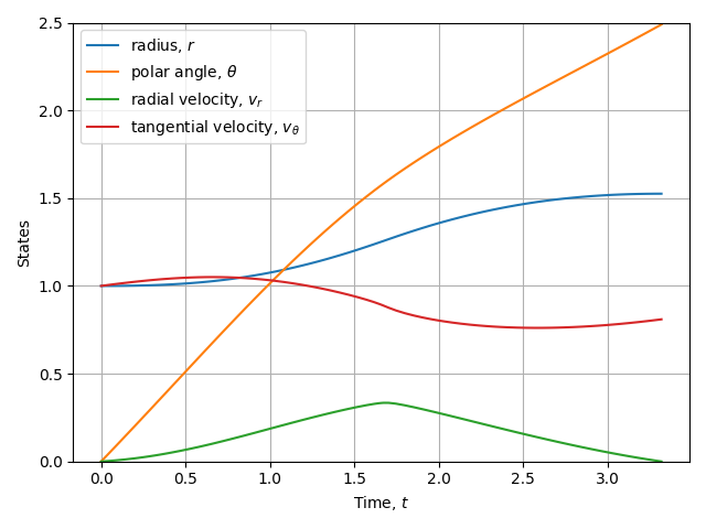
# figure 1: Plot states
plt.figure(1)
plt.plot(t, r, label=r"radius, $r$")
plt.plot(t, theta, label=r"polar angle, $\theta$")
plt.plot(t, v_r, label=r"radial velocity, $v_r$")
plt.plot(t, v_theta, label=r"tangential velocity, $v_\theta$")
plt.ylim([0, 2.5])
plt.ylabel("States")
plt.legend()
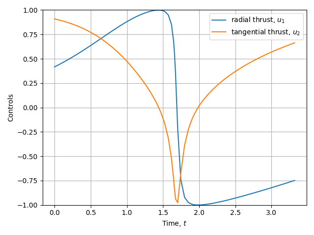
# figure 2: Plot control
plt.figure(2)
plt.plot(tc, control[0], label=r"radial thrust, $u_1$")
plt.plot(tc, control[1], label=r"tangential thrust, $u_2$")
plt.ylabel("Controls")
plt.legend()
plt.ylim([-1, 1])
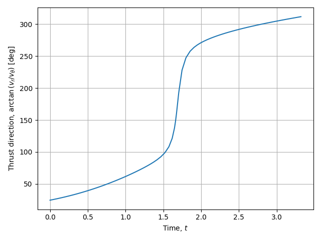
# figure 3: Thrust direction
plt.figure(3)
plt.plot(tc, 180 / pi * np.unwrap(np.arctan2(control[0], control[1])))
plt.ylabel(r"Thrust direction, $\arctan\left(v_r/v_\theta\right)$ [deg]")
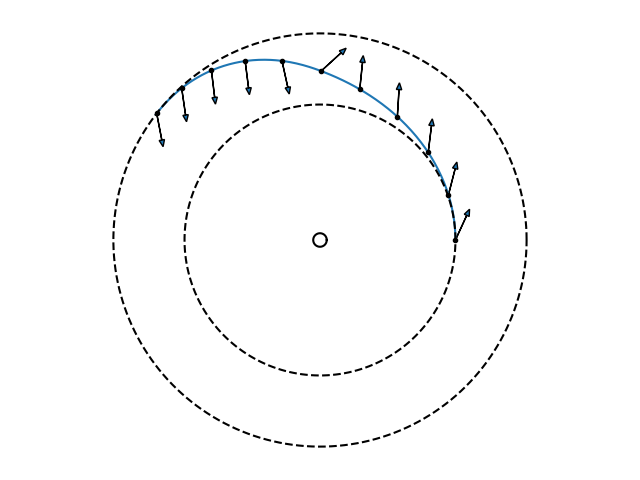
# figure 4: orbit
plt.figure(4)
# lgr doesn't find endpoint control, so need to fix up length of theta
m = len(u1)
v1 = np.cos(theta[:m]) * u1 - np.sin(theta[:m]) * u2
v2 = np.sin(theta[:m]) * u1 + np.cos(theta[:m]) * u2
plt.plot(x, y)
alpha = np.linspace(0, 2 * np.pi, num=200)
plt.plot(r[0] * np.cos(alpha), r[0] * np.sin(alpha), "k--")
plt.plot(r[-1] * np.cos(alpha), r[-1] * np.sin(alpha), "k--")
plt.plot(0.05 * np.cos(alpha), 0.05 * np.sin(alpha), "k")
for i in range(11):
j = round(i * (len(r) - 2) / 10)
plt.plot(x[j], y[j], ".k")
plt.arrow(
x[j],
y[j],
0.25 * v1[j],
0.25 * v2[j],
length_includes_head=True,
head_width=0.04,
head_length=0.05,
)
plt.axis("square")
plt.axis("equal")
plt.axis("off")
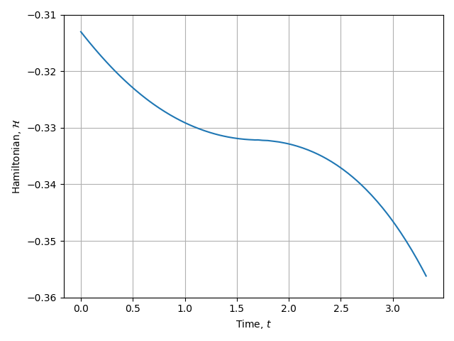
# figure 5: Hamiltonian
plt.figure(5)
hamiltonian = solution.phase[0].hamiltonian
plt.plot(tc, hamiltonian)
plt.ylabel(r"Hamiltonian, $\mathcal{H}$")
plt.ylim([-0.36, -0.31])
for i in range(5, 0, -1):
plt.figure(i)
if i != 4: # noqa: PLR2004
plt.xlabel("Time, $t$")
plt.grid()
plt.tight_layout()
def main() -> None:
"""Demonstrate the solution to the four state orbit raising optimal control problem."""
ocp = setup()
solution = ocp.solve()
plot_solution(solution)
plt.show()
if __name__ == "__main__":
main()
Text Output
******************************************************************************
This program contains Ipopt, a library for large-scale nonlinear optimization.
 Ipopt is released as open source code under the Eclipse Public License (EPL).
         For more information visit https://github.com/coin-or/Ipopt
******************************************************************************

Total number of variables............................:      581
                     variables with only lower bounds:        0
                variables with lower and upper bounds:      541
                     variables with only upper bounds:        0
Total number of equality constraints.................:      492
Total number of inequality constraints...............:        1
        inequality constraints with only lower bounds:        1
   inequality constraints with lower and upper bounds:        0
        inequality constraints with only upper bounds:        0


Number of Iterations....: 89

                                   (scaled)                 (unscaled)
Objective...............:  -1.5252776844830602e+00   -1.5252776844830602e+00
Dual infeasibility......:   1.8949139036395348e-12    1.8949139036395348e-12
Constraint violation....:   1.7175150190951172e-13    1.7175150190951172e-13
Variable bound violation:   0.0000000000000000e+00    0.0000000000000000e+00
Complementarity.........:   5.0000000000105322e-21    5.0000000000105322e-21
Overall NLP error.......:   1.8949139036395348e-12    1.8949139036395348e-12


Number of objective function evaluations             = 110
Number of objective gradient evaluations             = 90
Number of equality constraint evaluations            = 110
Number of inequality constraint evaluations          = 110
Number of equality constraint Jacobian evaluations   = 90
Number of inequality constraint Jacobian evaluations = 90
Number of Lagrangian Hessian evaluations             = 89
Total seconds in IPOPT (w/o function evaluations)    =      1.529
Total seconds in NLP function evaluations            =      0.750

EXIT: Solved To Acceptable Level.
Plots
State Vector
Control Vector
Thrust Direction
Orbital Transfer Trajectory
Hamiltonian