The Goddard Problem (One Phase)
For a description of the one-phase Goddard rocket problem, see the JupyterLab notebook documentation for this problem.
It turns out that this problem as a singular arc, and a better solution can be obtained by solving the problem in three phases, where the singular arc conditions are imposed as a path constraint in the middle phase. See the three phase solution as a Python script or as a JupyterLab notebook.
This example script has user-defined methods for computing the first and second derivatives of the objective and continuous functions. User-defined derivatives can be faster to compute than derivatives computed by automatic differentiation, but not by a large factor. Because for most problems as much time is spent in the Ipopt solver as in derivative functions evaluation, even a substantial speedup in derivative evaluation may not result in a significant speedup in the overall solution time, and so it’s almost never worth the effort to implement user-defined derivatives.
The python script in this example can be executed from the command line with:
$ python -m yapss.examples.goddard_problem_1_phase
Functions
YAPSS solution of the Goddard rocket problem with a single phase.
Code
"""
YAPSS solution of the Goddard rocket problem with a single phase.
"""
# Allow uppercase variables
# ruff: noqa: N806
__all__ = ["main", "plot_solution", "setup"]
# third party imports
import matplotlib.pyplot as plt
from yapss import (
ContinuousArg,
ContinuousHessianArg,
ContinuousJacobianArg,
ObjectiveArg,
ObjectiveGradientArg,
ObjectiveHessianArg,
Problem,
Solution,
)
# package imports
from yapss.math import exp
def setup() -> Problem:
"""Set up the Goddard Rocket Problem as an optimal control problem.
Returns
-------
Problem
The Goddard Rocket Problem as an optimal control problem.
"""
h0, v0, m0 = 0, 0, 3
mf = 1
hmin, hmax = 0, 30000
vmin, vmax = 0, 15000
t0 = 0
tfMin, tfMax = 20, 100
ocp = Problem(name="One phase Goddard Rocket Problem", nx=[3], nu=[1])
def objective(arg: ObjectiveArg) -> None:
"""Goddard Rocket Problem objective function."""
arg.objective = arg.phase[0].final_state[0]
def continuous(arg: ContinuousArg) -> None:
"""Goddard Rocket Problem dynamics."""
auxdata = arg.auxdata
h, v, m = arg.phase[0].state
(T,) = arg.phase[0].control
dynamics = arg.phase[0].dynamics
v_dot = (T - auxdata.sigma * v**2 * exp(-h / auxdata.h0)) / m - auxdata.g
m_dot = -T / auxdata.c
dynamics[0] = v
dynamics[1] = v_dot
dynamics[2] = m_dot
# Optional first derivative functions
def objective_gradient(arg: ObjectiveGradientArg) -> None:
"""Objective gradient for the Goddard Rocket Problem."""
arg.gradient[(0, "xf", 0)] = 1
def continuous_jacobian(arg: ContinuousJacobianArg) -> None:
"""Jacobian of the dynamics for the Goddard Rocket Problem."""
auxdata = arg.auxdata
sigma = auxdata.sigma
h0 = auxdata.h0
c = auxdata.c
h, v, m = arg.phase[0].state
(T,) = arg.phase[0].control
D_div_v2 = sigma * exp(-h / h0)
D_div_v = D_div_v2 * v
D = D_div_v * v
jacobian = arg.phase[0].jacobian
jacobian[("f", 0), ("x", 1)] = 1 + 0 * v
jacobian[("f", 1), ("x", 0)] = D / (h0 * m)
jacobian[("f", 1), ("x", 1)] = -2 * D_div_v / m
jacobian[("f", 1), ("x", 2)] = -(T - D) / m**2
jacobian[("f", 1), ("u", 0)] = 1 / m
jacobian[("f", 2), ("u", 0)] = -1 / c + 0 * v
# Optional second derivative functions
def objective_hessian(_: ObjectiveHessianArg) -> None:
"""Hessian of the objective function for the Goddard Rocket Problem."""
return
def continuous_hessian(arg: ContinuousHessianArg) -> None:
"""Hessian of the dynamics for the Goddard Rocket Problem."""
auxdata = arg.auxdata
sigma = auxdata.sigma
h0 = auxdata.h0
for p in arg.phase_list:
h, v, m = arg.phase[p].state
(T,) = arg.phase[p].control
D_div_v2 = sigma * exp(-h / h0)
D_div_v = D_div_v2 * v
D = D_div_v * v
hessian = arg.phase[0].hessian
hessian[("f", 1), ("x", 0), ("x", 0)] = -D / (h0**2 * m)
hessian[("f", 1), ("x", 0), ("x", 1)] = 2 * D_div_v / (h0 * m)
hessian[("f", 1), ("x", 0), ("x", 2)] = -D / (h0 * m**2)
hessian[("f", 1), ("x", 1), ("x", 1)] = -2 * D_div_v2 / m
hessian[("f", 1), ("x", 1), ("x", 2)] = 2 * D_div_v / m**2
hessian[("f", 1), ("x", 2), ("x", 2)] = 2 * (T - D) / m**3
hessian[("f", 1), ("x", 2), ("u", 0)] = -1 / m**2
# physical constants
auxdata = ocp.auxdata
auxdata.Tm = Tm = 193.044
auxdata.g = 32.174
auxdata.sigma = 5.49153484923381010e-05
auxdata.c = 1580.9425279876559
auxdata.h0 = 23800
functions = ocp.functions
functions.objective = objective
functions.objective_gradient = objective_gradient
functions.objective_hessian = objective_hessian
functions.continuous = continuous
functions.continuous_jacobian = continuous_jacobian
functions.continuous_hessian = continuous_hessian
# bounds
bounds = ocp.bounds.phase[0]
bounds.initial_time.lower = bounds.initial_time.upper = t0
bounds.final_time.lower = tfMin
bounds.final_time.upper = tfMax
bounds.initial_state.lower[:] = bounds.initial_state.upper[:] = [h0, v0, m0]
bounds.state.lower[:] = [hmin, vmin, mf]
bounds.state.upper[:] = [hmax, vmax, m0]
bounds.final_state.lower[:] = [hmin, vmin, mf]
bounds.final_state.upper[:] = [hmax, vmax, mf]
bounds.control.lower[:] = (0,)
bounds.control.upper[:] = (Tm,)
# guess
phase = ocp.guess.phase[0]
phase.time = (t0, tfMax)
phase.state = ((h0, h0), (v0, v0), (m0, mf))
phase.control = ((0, Tm),)
# solver settings
ocp.derivatives.order = "second"
ocp.derivatives.method = "auto"
# ipopt options
ocp.ipopt_options.tol = 1e-20
ocp.ipopt_options.print_level = 3
ocp.scale.objective = -1
# TODO: Fails if all scales are integers
ocp.scale.phase[0].state = ocp.scale.phase[0].dynamics = 18_000, 800, 3
ocp.scale.phase[0].time = 30
return ocp
def plot_solution(solution: Solution) -> None:
"""Plot solution to the Goddard Rocket Problem.
Parameters
----------
solution : Solution
The solution to the Goddard Rocket Problem.
"""
# extract information from solution
time = solution.phase[0].time
time_c = solution.phase[0].time_c
h, v, m = solution.phase[0].state
(T,) = solution.phase[0].control
hamiltonian = solution.phase[0].hamiltonian
t0 = solution.phase[0].initial_time
tf = solution.phase[0].final_time
# thrust
plt.figure(1)
plt.plot(time_c, T)
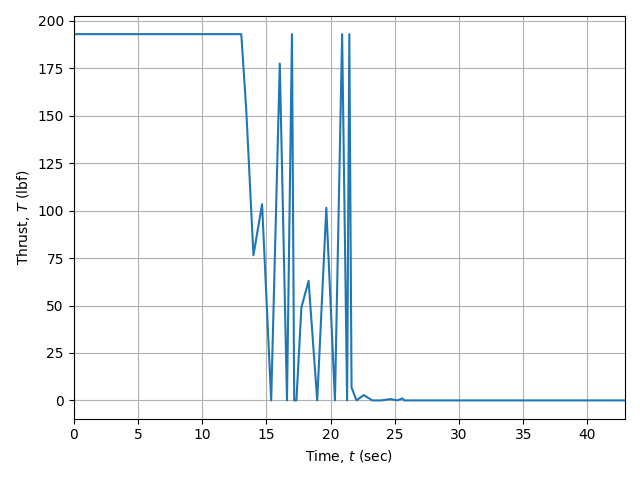
plt.ylabel("Thrust, $T$ (lbf)")
# altitude
plt.figure(2)
plt.plot(time, h)
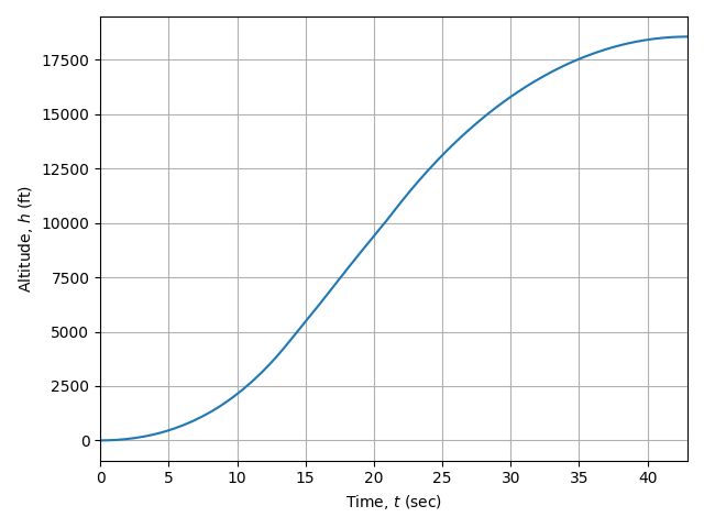
plt.ylabel("Altitude, $h$ (ft)")
# velocity
plt.figure(3)
plt.plot(time, v)
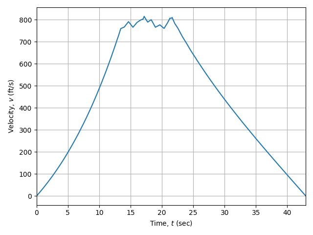
plt.ylabel("Velocity, $v$ (ft/s)")
# mass
plt.figure(4)
plt.plot(time, m)
plt.ylabel("Mass, $m$ (slugs)")
# hamiltonian
plt.figure(5)
plt.plot(time_c, hamiltonian)
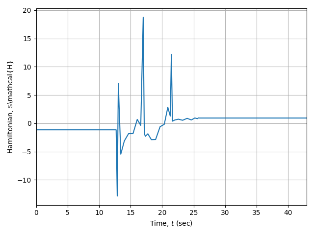
plt.ylabel(r"Hamiltonian, $\mathcal{H}")
for i in range(1, 6):
plt.figure(i)
plt.xlabel("Time, $t$ (sec)")
plt.xlim([t0, tf])
plt.tight_layout()
plt.grid()
def main() -> None:
"""Demonstrate the solution to the Goddard Rocket Problem (1 Phase)."""
problem = setup()
solution = problem.solve()
plot_solution(solution)
plt.show()
if __name__ == "__main__":
main()
Text Output
******************************************************************************
This program contains Ipopt, a library for large-scale nonlinear optimization.
 Ipopt is released as open source code under the Eclipse Public License (EPL).
         For more information visit https://github.com/coin-or/Ipopt
******************************************************************************

Total number of variables............................:      391
                     variables with only lower bounds:        0
                variables with lower and upper bounds:      361
                     variables with only upper bounds:        0
Total number of equality constraints.................:      300
Total number of inequality constraints...............:        1
        inequality constraints with only lower bounds:        1
   inequality constraints with lower and upper bounds:        0
        inequality constraints with only upper bounds:        0


Number of Iterations....: 71

                                   (scaled)                 (unscaled)
Objective...............:  -1.8563367158669407e+04    1.8563367158669407e+04
Dual infeasibility......:   5.4569682106375694e-11    1.8189894035458565e-11
Constraint violation....:   9.4890613884975513e-14    1.7080310499295592e-09
Variable bound violation:   1.9304399927477789e-06    1.9304399927477789e-06
Complementarity.........:   5.0047179600681232e-21    5.0047179600681232e-21
Overall NLP error.......:   3.0230044705216128e-11    1.7080310499295592e-09


Number of objective function evaluations             = 77
Number of objective gradient evaluations             = 72
Number of equality constraint evaluations            = 77
Number of inequality constraint evaluations          = 77
Number of equality constraint Jacobian evaluations   = 72
Number of inequality constraint Jacobian evaluations = 72
Number of Lagrangian Hessian evaluations             = 71
Total seconds in IPOPT (w/o function evaluations)    =      0.665
Total seconds in NLP function evaluations            =      0.161

EXIT: Solved To Acceptable Level.
Plots
Thrust
Altitude
Velocity
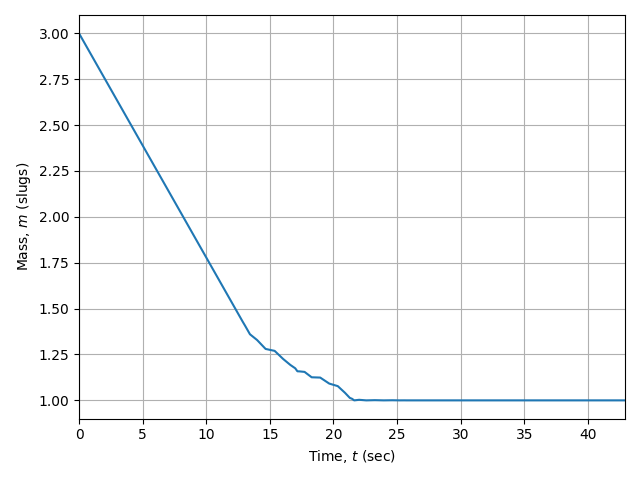
Mass
Hamiltonian
The fact that the Hamiltonian is not constant even though the dynamics and cost integrand are time-invariant is a good indication that there is a singular arc. Indeed, this problem does have a singular arc in the middle of the trajectory.