Rosenbrock Function

For a solution to the Rosenbrock function minimization problem using a Python script instead of a notebook, see the Python script documentation.

Description

YAPSS is primarily an optimal control problem solver, but can solve parameter optimization problems as well — a parameter optimization problem is just an optimal control problem with no dynamics!

The cost function to be minimized is the Rosenbrock function [1],

\[J = f(x) = 100 (x_1 - x_0 ^ 2) ^ 2 + (1 - x_0) ^ 2\]

is a function often used to test optimization algorithms. Because the function is the sum of two squares, it’s straightforward to verify that the Rosenbrock function has its global minimum at \(x = (1,1)\), since

\[\begin{split}\begin{aligned} f(x) & = 0,\quad x = (1,1) \\ f(x) & > 0,\quad x \ne (1,1) \end{aligned}\end{split}\]

The global minimum lies in a narrow parabolic-shaped valley, making the minimum difficult to find.

We can make a contour plot of the function using Matplotlib:

import numpy as np
from matplotlib import pyplot as plt

x0 = np.linspace(-2, 2, 400)
x1 = np.linspace(-1, 3, 400)
x0_grid, x1_grid = np.meshgrid(x0, x1)
f = 100 * (x1_grid - x0_grid**2) ** 2 + (1 - x0_grid) ** 2
levels = [1, 3, 10, 30, 100, 300, 1000, 3000]
cp = plt.contour(x0, x1, f, levels, colors="black", linewidths=0.5)
plt.clabel(cp, inline=1, fontsize=8)
plt.plot(1, 1, ".r", markersize=5)
plt.xlabel(r"$x_0$")
plt.ylabel(r"$x_1$")
plt.xticks(range(-2, 3))
plt.yticks(range(-1, 4))
plt.tight_layout()

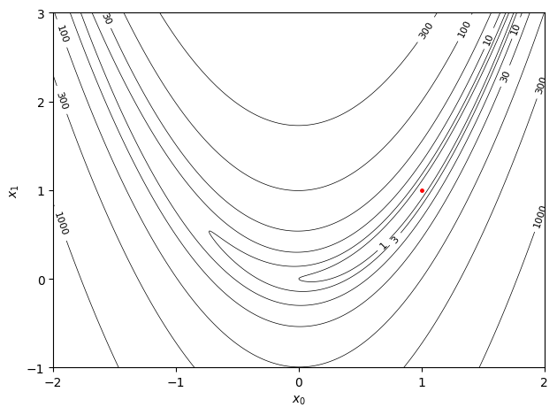
The minimum is marked by the red dot in the figure above.

YAPSS Solution

To find the minimum, first instantiate the problem with no phase and two parameters:

from yapss import Problem

problem = Problem(name="Rosenbrock", nx=[], ns=2)

Define the objective function:

def objective(arg):
    x0, x1 = arg.parameter
    arg.objective = 100 * (x1 - x0**2) ** 2 + (1 - x0) ** 2


problem.functions.objective = objective

Define the initial guess:

problem.guess.parameter = [-2.0, 2.0]

For the optimization, use first and second derivatives of the objective function, found using automatic differentiation. Set the tol Ipopt option to 1e-10 (default is 1e-8).

problem.derivatives.order = "second"
problem.derivatives.method = "auto"
problem.ipopt_options.tol = 1e-10

Set Ipopt options to control the amount of printout from Ipopt:

# some output, but don't print iterations
problem.ipopt_options.print_level = 3

# suppress the Ipopt banner
problem.ipopt_options.sb = "yes"

# don't print out the Ipopt options
problem.ipopt_options.print_user_options = "no"

All that remains is to solve the problem:

solution = problem.solve()

Total number of variables............................:        2
                     variables with only lower bounds:        0
                variables with lower and upper bounds:        0
                     variables with only upper bounds:        0
Total number of equality constraints.................:        0
Total number of inequality constraints...............:        0
        inequality constraints with only lower bounds:        0
   inequality constraints with lower and upper bounds:        0
        inequality constraints with only upper bounds:        0


Number of Iterations....: 26

                                   (scaled)                 (unscaled)
Objective...............:   0.0000000000000000e+00    0.0000000000000000e+00
Dual infeasibility......:   0.0000000000000000e+00    0.0000000000000000e+00
Constraint violation....:   0.0000000000000000e+00    0.0000000000000000e+00
Variable bound violation:   0.0000000000000000e+00    0.0000000000000000e+00
Complementarity.........:   0.0000000000000000e+00    0.0000000000000000e+00
Overall NLP error.......:   0.0000000000000000e+00    0.0000000000000000e+00


Number of objective function evaluations             = 61
Number of objective gradient evaluations             = 27
Number of equality constraint evaluations            = 0
Number of inequality constraint evaluations          = 0
Number of equality constraint Jacobian evaluations   = 0
Number of inequality constraint Jacobian evaluations = 0
Number of Lagrangian Hessian evaluations             = 26
Total seconds in IPOPT (w/o function evaluations)    =      0.011
Total seconds in NLP function evaluations            =      0.013

EXIT: Optimal Solution Found.

We can print out the solution with the code:

print(solution)

<yapss._private.solution.Solution> object
    Name: Rosenbrock
    Ipopt Status Code: 0
    Status Message: Optimal Solution Found
    Objective Value: 0.0

x_opt = solution.parameter
print(f"The optimal solution is at the point x = {x_opt}")

The optimal solution is at the point x = [1. 1.]

References

[1]

H. H. Rosenbrock. An automatic method for finding the greatest or least value of a function. The Computer Journal, 3(3):175–184, 1960. doi:10.1093/comjnl/3.3.175.