Brachistochrone (Minimal Implementation)
For a description of the brachistochrone problem with constraints as in this script, see the JupyterLab notebook Tutorial Example.
This script provides a minimal implementation of the brachistochrone problem, that is, without providing user-defined derivatives. (User-defined derivatives are almost never necessary.) For a script that implements the brachistochrone problem with user-defined derivatives, see the example implementation of the brachistochrone problem with user defined derivatives..
The python script in this example can be executed from the command line with:
$ python -m yapss.examples.brachistochrone_minimal
Functions
Minimal YAPSS solution of the brachistochrone optimal control problem.
Code
"""
Minimal YAPSS solution of the brachistochrone optimal control problem.
"""
__all__ = ["main", "plot_solution", "setup"]
# third party imports
import matplotlib.pyplot as plt
from yapss import ContinuousArg, ObjectiveArg, Problem, Solution
# package imports
from yapss.math import cos, sin
def setup() -> Problem:
"""Set up the brachistochrone optimal control problem.
Returns
-------
Problem
The brachistochrone optimal control problem.
"""
# Initialize optimal control problem
problem = Problem(name="Brachistochrone", nx=[3], nu=[1])
g0 = 32.174
def objective(arg: ObjectiveArg) -> None:
"""Objective callback function. Objective is to minimize final time."""
arg.objective = arg.phase[0].final_time
# continuous function
def continuous(arg: ContinuousArg) -> None:
"""Continuous callback function."""
x, y, v = arg.phase[0].state
(u,) = arg.phase[0].control
arg.phase[0].dynamics = v * cos(u), v * sin(u), g0 * sin(u)
problem.functions.objective = objective
problem.functions.continuous = continuous
# bounds
bounds = problem.bounds.phase[0]
bounds.initial_time.lower = bounds.initial_time.upper = 0.0
bounds.initial_state.lower[:] = bounds.initial_state.upper[:] = 0.0
bounds.final_state.lower[0] = bounds.final_state.upper[0] = 1.0
bounds.state.lower[:] = 0.0
bounds.state.upper[:] = 10.0
# guess
phase = problem.guess.phase[0]
phase.time = [0.0, 1.0]
phase.state = [[0.0, 1.0], [0.0, 1.0], [0.0, 10.0]]
phase.control = [[0.0, 0.0]]
problem.derivatives.method = "auto"
# ipopt options
problem.ipopt_options.print_level = 3
return problem
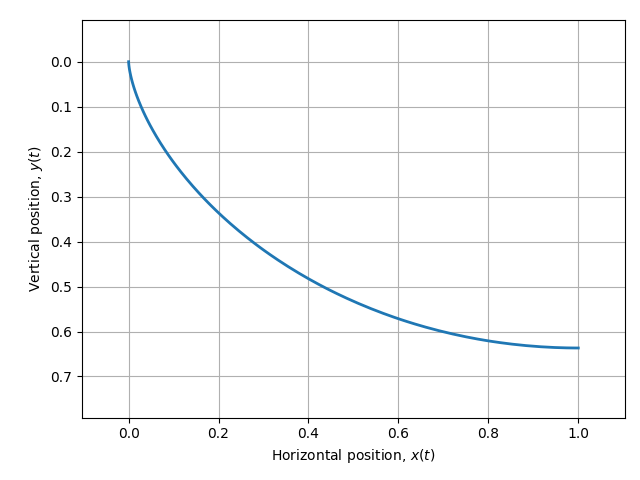
def plot_solution(solution: Solution) -> None:
"""Plot the solution to the brachistochrone optimal control problem.
Parameters
----------
solution : Solution
The solution to the brachistochrone optimal control problem.
"""
# extract solution
x, y, _ = solution.phase[0].state
# plot
plt.figure()
plt.plot(x, y, linewidth=2)
plt.xlabel("Horizontal position, $x(t)$")
plt.ylabel("Vertical position, $y(t)$")
plt.axis("equal")
plt.xlim([0.0, 1.0])
plt.ylim([0.8, -0.1])
plt.tight_layout()
plt.grid()
def main() -> None:
"""Demonstrate the solution to the brachistochrone optimal control problem."""
ocp = setup()
solution = ocp.solve()
print(f"\nObjective = {solution.objective}")
plot_solution(solution)
plt.show()
if __name__ == "__main__":
main()
Text Output
******************************************************************************
This program contains Ipopt, a library for large-scale nonlinear optimization.
 Ipopt is released as open source code under the Eclipse Public License (EPL).
         For more information visit https://github.com/coin-or/Ipopt
******************************************************************************

Total number of variables............................:      391
                     variables with only lower bounds:        0
                variables with lower and upper bounds:      269
                     variables with only upper bounds:        0
Total number of equality constraints.................:      300
Total number of inequality constraints...............:        1
        inequality constraints with only lower bounds:        1
   inequality constraints with lower and upper bounds:        0
        inequality constraints with only upper bounds:        0


Number of Iterations....: 27

                                   (scaled)                 (unscaled)
Objective...............:   3.1248013070855907e-01    3.1248013070855907e-01
Dual infeasibility......:   3.5953151805538652e-12    3.5953151805538652e-12
Constraint violation....:   1.9927504091299397e-11    1.9927504091299397e-11
Variable bound violation:   0.0000000000000000e+00    0.0000000000000000e+00
Complementarity.........:   1.0000000000606486e-11    1.0000000000606486e-11
Overall NLP error.......:   1.9927504091299397e-11    1.9927504091299397e-11


Number of objective function evaluations             = 28
Number of objective gradient evaluations             = 28
Number of equality constraint evaluations            = 28
Number of inequality constraint evaluations          = 28
Number of equality constraint Jacobian evaluations   = 28
Number of inequality constraint Jacobian evaluations = 28
Number of Lagrangian Hessian evaluations             = 27
Total seconds in IPOPT (w/o function evaluations)    =      0.260
Total seconds in NLP function evaluations            =      0.062

EXIT: Optimal Solution Found.

Objective = 0.31248013070855907
Plots
State Trajectory