The Isoperimetric Problem
For a description of the isoperimetric problem, see the JupyterLab notebook documentation for this problem.
The python script in this example can be executed from the command line with:
$ python -m yapss.examples.isoperimetric
Functions
YAPSS solution of the isoperimetric problem.
Code
"""
YAPSS solution of the isoperimetric problem.
"""
__all__ = ["main", "plot_solution", "setup"]
# standard library imports
import math
# package imports
import numpy as np
# third party imports
from matplotlib import pyplot as plt
from scipy.interpolate import interp1d
from yapss import ContinuousArg, DiscreteArg, ObjectiveArg, Problem, Solution
def setup() -> Problem:
"""Set up the isoperimetric optimization problem.
Returns
-------
Problem
The isoperimetric optimization problem.
"""
# problem has 1 phase, with 2 states, 2 controls, 1 path constraint, and 3
# integrals. There are four constraints: 2 to constrain the curved to be closed,
# and 2 to constrain the centroid of the curve to be at the origin.
ocp = Problem(name="Isoperimetric Problem", nx=[2], nu=[2], nq=[3], nh=[1], nd=4)
def objective(arg: ObjectiveArg) -> None:
"""Objective callback function."""
arg.objective = arg.phase[0].integral[0]
def continuous(arg: ContinuousArg) -> None:
"""Continuous callback function."""
x, y = arg.phase[0].state
ux, uy = arg.phase[0].control
arg.phase[0].dynamics[:] = ux, uy
arg.phase[0].path[0] = ux**2 + uy**2
arg.phase[0].integrand[0] = (y * ux - x * uy) / 2
arg.phase[0].integrand[1] = x
arg.phase[0].integrand[2] = y
def discrete(arg: DiscreteArg) -> None:
"""Discrete callback function."""
arg.discrete[:2] = arg.phase[0].final_state - arg.phase[0].initial_state
arg.discrete[2:4] = arg.phase[0].integral[1:]
ocp.functions.objective = objective
ocp.functions.continuous = continuous
ocp.functions.discrete = discrete
# bounds
bounds = ocp.bounds.phase[0]
bounds.path.lower[0] = bounds.path.upper[0] = 1
bounds.initial_time.lower = bounds.initial_time.upper = 0.0
bounds.final_time.lower = bounds.final_time.upper = 1.0
bounds.state.lower[:] = -10
bounds.state.upper[:] = +10
bounds.control.lower[:] = -2
bounds.control.upper[:] = +2
ocp.bounds.discrete.lower = ocp.bounds.discrete.upper = [0, 0, 0, 0]
ocp.bounds.discrete.lower[2:] = -1e-4
ocp.bounds.discrete.upper[2:] = +1e-4
# guess
guess = ocp.guess.phase[0]
guess.time = [0.0, 0.25, 0.5, 0.75, 1.0]
guess.state = [
[1.0, 0.0, -1.0, 0.0, 1.0],
[0.0, -1.0, 0.0, 1.0, 0.0],
]
# mesh
m, n = 3, 15
ocp.mesh.phase[0].collocation_points = m * (n,)
ocp.mesh.phase[0].fraction = m * (1.0 / m,)
# set objective scale to maximize objective
ocp.scale.objective = -1
# yapss and ipopt options
ocp.derivatives.method = "auto"
ocp.derivatives.order = "second"
ocp.ipopt_options.tol = 1e-20
ocp.ipopt_options.print_level = 3
return ocp
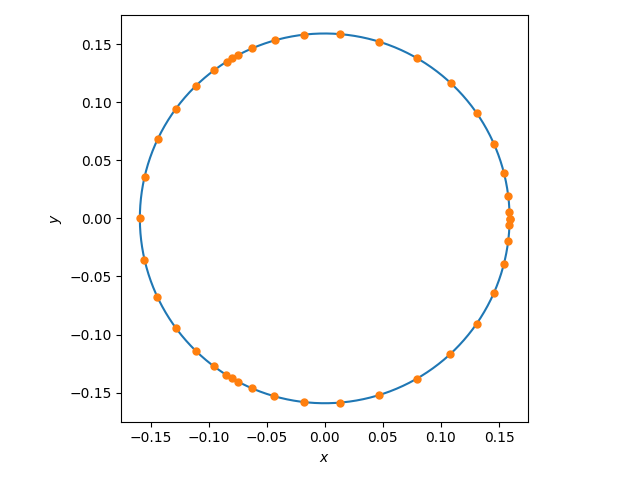
def plot_solution(solution: Solution) -> None:
"""Plot the solution to the isoperimetric problem.
The collocation points are shown as dots, and the curve is interpolated between
points with a cubic spline.
Parameters
----------
solution: Solution
The solution to the isoperimetric problem.
"""
plt.figure(1)
plt.clf()
x, y = solution.phase[0].state
s = solution.phase[0].time
sp = np.linspace(0, 1, 500)
xp = interp1d(s, x, kind="cubic")(sp)
yp = interp1d(s, y, kind="cubic")(sp)
plt.plot(xp, yp)
plt.plot(x, y, ".", markersize=10)
plt.xlabel("$x$")
plt.ylabel("$y$")
plt.axis("square")
plt.tight_layout()
def main() -> None:
"""Demonstrate the solution to the isoperimetric problem."""
problem = setup()
solution = problem.solve()
# print the solution
area = solution.objective
area_ideal = 1 / (4 * math.pi)
print(f"\n\nMaximum area = {area} (Should be 1 / (4 pi) = {area_ideal})")
print(f"Relative error in solution = {abs(area - area_ideal) / area_ideal}")
# plot the solution
plot_solution(solution)
plt.show()
if __name__ == "__main__":
main()
Text Output
******************************************************************************
This program contains Ipopt, a library for large-scale nonlinear optimization.
 Ipopt is released as open source code under the Eclipse Public License (EPL).
         For more information visit https://github.com/coin-or/Ipopt
******************************************************************************

Total number of variables............................:      181
                     variables with only lower bounds:        0
                variables with lower and upper bounds:      172
                     variables with only upper bounds:        0
Total number of equality constraints.................:      138
Total number of inequality constraints...............:        3
        inequality constraints with only lower bounds:        1
   inequality constraints with lower and upper bounds:        2
        inequality constraints with only upper bounds:        0


Number of Iterations....: 68

                                   (scaled)                 (unscaled)
Objective...............:  -7.9577471545947673e-02    7.9577471545947673e-02
Dual infeasibility......:   2.8897348699173663e-17    2.8897348699173663e-17
Constraint violation....:   6.9271303103357607e-15    6.9271303103357607e-15
Variable bound violation:   0.0000000000000000e+00    0.0000000000000000e+00
Complementarity.........:   5.0000000000000012e-21    5.0000000000000012e-21
Overall NLP error.......:   6.9271303103357607e-15    6.9271303103357607e-15


Number of objective function evaluations             = 121
Number of objective gradient evaluations             = 69
Number of equality constraint evaluations            = 121
Number of inequality constraint evaluations          = 121
Number of equality constraint Jacobian evaluations   = 69
Number of inequality constraint Jacobian evaluations = 69
Number of Lagrangian Hessian evaluations             = 68
Total seconds in IPOPT (w/o function evaluations)    =      0.351
Total seconds in NLP function evaluations            =      0.173

EXIT: Solved To Acceptable Level.


Maximum area = 0.07957747154594767 (Should be 1 / (4 pi) = 0.07957747154594767)
Relative error in solution = 0.0
Plots