The Goddard Problem (Three Phases)
For a description of the one-phase Goddard rocket problem, see the JupyterLab notebook documentation for this problem.
This problem has three phases because there is a singular arc in the solution. In the middle phase, the singular arc conditions are imposed as a path constraint. This results in a significantly better solution than the one-phase solution. See the one phase solution as a Python script or as a JupyterLab notebook.
This example script has user-defined methods for computing the first and second derivatives of the objective and continuous functions. User-defined derivatives can be faster to compute than derivatives computed by automatic differentiation, but not by a large factor. Because for most problems as much time is spent in the Ipopt solver as in derivative functions evaluation, even a substantial speedup in derivative evaluation may not result in a significant speedup in the overall solution time, and so it’s almost never worth the effort to implement user-defined derivatives.
The python script in this example can be executed from the command line with:
$ python -m yapss.examples.goddard_problem_3_phase
Functions
YAPSS solution of the Goddard rocket problem with three phases (one a singular arc).
Code
"""
YAPSS solution of the Goddard rocket problem with three phases (one a singular arc).
"""
# Allow uppercase variables
# ruff: noqa: N806
__all__ = ["main", "plot_solution", "setup"]
# third party imports
import matplotlib.pyplot as plt
from yapss import (
ContinuousArg,
ContinuousHessianArg,
ContinuousJacobianArg,
DiscreteArg,
DiscreteHessianArg,
DiscreteJacobianArg,
ObjectiveArg,
ObjectiveGradientArg,
ObjectiveHessianArg,
Problem,
Solution,
)
# package imports
from yapss.math import exp
def setup() -> Problem:
"""Set up the Goddard Rocket Problem optimal control problem.
Returns
-------
yapss.Problem:
Optimal control problem object
"""
ocp = Problem(
name="Goddard Rocket Problem with Singular Arc",
nx=[3, 3, 3],
nu=[1, 1, 1],
nh=[0, 1, 0],
nq=[0, 0, 0],
nd=8,
)
# callback functions
def objective(arg: ObjectiveArg) -> None:
"""Goddard Rocket Problem objective function."""
arg.objective = arg.phase[2].final_state[0]
def objective_gradient(arg: ObjectiveGradientArg) -> None:
"""Gradient of Goddard Rocket Problem objective function."""
arg.gradient[(2, "xf", 0)] = 1
def objective_hessian(_: ObjectiveHessianArg) -> None:
"""Hessian of Goddard Rocket Problem objective function."""
# noinspection PyPep8Naming
def continuous(arg: ContinuousArg) -> None:
"""Goddard Rocket Problem dynamics and path functions."""
auxdata = arg.auxdata
sigma = auxdata.sigma
h0 = auxdata.h0
c = auxdata.c
g0 = auxdata.g
for p in arg.phase_list:
(h, v, mass) = arg.phase[p].state
(T,) = arg.phase[p].control
D = sigma * v**2.0 * exp(-h / h0)
h_dot = v
v_dot = (T - D) / mass - g0
m_dot = -T / c
arg.phase[p].dynamics[:] = (h_dot, v_dot, m_dot)
if p == 1:
arg.phase[p].path[:] = (mass * g0 - (1 + v / c) * D,)
# noinspection PyPep8Naming,PyPep8Naming,PyPep8Naming,PyPep8Naming
def continuous_jacobian(arg: ContinuousJacobianArg) -> None:
"""Jacobian of Goddard Rocket Problem dynamics and path functions."""
auxdata = arg.auxdata
sigma = auxdata.sigma
h0 = auxdata.h0
c = auxdata.c
g0 = auxdata.g
for p in arg.phase_list:
h, v, mass = arg.phase[p].state
(T,) = arg.phase[p].control
D_div_v2 = sigma * exp(-h / h0)
D_div_v = D_div_v2 * v
D = D_div_v * v
jacobian = arg.phase[p].jacobian
jacobian[("f", 0), ("x", 1)] = 1
jacobian[("f", 1), ("x", 0)] = D / (h0 * mass)
jacobian[("f", 1), ("x", 1)] = -2 * D_div_v / mass
jacobian[("f", 1), ("x", 2)] = -(T - D) / mass**2
jacobian[("f", 1), ("u", 0)] = 1 / mass
jacobian[("f", 2), ("u", 0)] = -1 / c
if p == 1:
jacobian[("h", 0), ("x", 0)] = D * (1 + v / c) / h0
jacobian[("h", 0), ("x", 1)] = D * (-3 / c) - 2 * D_div_v
jacobian[("h", 0), ("x", 2)] = g0
# noinspection PyPep8Naming
def continuous_hessian(arg: ContinuousHessianArg) -> None:
"""Hessian of Goddard Rocket Problem dynamics and path functions."""
auxdata = arg.auxdata
sigma = auxdata.sigma
h0 = auxdata.h0
c = auxdata.c
for p in arg.phase_list:
h, v, mass = arg.phase[p].state
(T,) = arg.phase[p].control
D_div_v2 = sigma * exp(-h / h0)
D_div_v = D_div_v2 * v
D = D_div_v * v
hessian = arg.phase[p].hessian
hessian[("f", 1), ("x", 0), ("x", 0)] = -D / (h0**2 * mass)
hessian[("f", 1), ("x", 0), ("x", 1)] = 2 * D_div_v / (h0 * mass)
hessian[("f", 1), ("x", 0), ("x", 2)] = -D / (h0 * mass**2)
hessian[("f", 1), ("x", 1), ("x", 1)] = -2 * D_div_v2 / mass
hessian[("f", 1), ("x", 1), ("x", 2)] = 2 * D_div_v / mass**2
hessian[("f", 1), ("x", 2), ("x", 2)] = 2 * (T - D) / mass**3
hessian[("f", 1), ("x", 2), ("u", 0)] = -1 / mass**2
if p == 1:
hessian[("h", 0), ("x", 0), ("x", 0)] = -D * (c + v) / (c * h0**2)
hessian[("h", 0), ("x", 0), ("x", 1)] = D_div_v * (2 * c + 3 * v) / (c * h0)
hessian[("h", 0), ("x", 1), ("x", 1)] = -2 * D_div_v2 * (c + 3 * v) / c
def discrete(arg: DiscreteArg) -> None:
"""Goddard Rocket Problem discrete constraint function."""
phase = arg.phase
arg.discrete = [
phase[0].final_time - phase[1].initial_time,
*(phase[0].final_state - phase[1].initial_state),
phase[1].final_time - phase[2].initial_time,
*(phase[1].final_state - phase[2].initial_state),
]
def discrete_jacobian(arg: DiscreteJacobianArg) -> None:
"""Jacobian of Goddard Rocket Problem discrete constraint function."""
jac = arg.jacobian
jac[0, (0, "tf", 0)] = 1
jac[0, (1, "t0", 0)] = -1
jac[1, (0, "xf", 0)] = 1
jac[1, (1, "x0", 0)] = -1
jac[2, (0, "xf", 1)] = 1
jac[2, (1, "x0", 1)] = -1
jac[3, (0, "xf", 2)] = 1
jac[3, (1, "x0", 2)] = -1
jac[4, (1, "tf", 0)] = 1
jac[4, (2, "t0", 0)] = -1
jac[5, (1, "xf", 0)] = 1
jac[5, (2, "x0", 0)] = -1
jac[6, (1, "xf", 1)] = 1
jac[6, (2, "x0", 1)] = -1
jac[7, (1, "xf", 2)] = 1
jac[7, (2, "x0", 2)] = -1
def discrete_hessian(_: DiscreteHessianArg) -> None:
"""Hessian of Goddard Rocket Problem discrete constraint function."""
# Initial conditions
h0 = 0
v0 = 0
m0 = 3
mf = 1
# physical constants
ocp.auxdata.Tm = Tm = 193.044
ocp.auxdata.g = 32.174
ocp.auxdata.sigma = 5.49153484923381010e-05
ocp.auxdata.c = 1580.9425279876559
ocp.auxdata.h0 = 23800
# user functions
ocp.functions.continuous = continuous
ocp.functions.continuous_jacobian = continuous_jacobian
ocp.functions.continuous_hessian = continuous_hessian
ocp.functions.objective = objective
ocp.functions.objective_gradient = objective_gradient
ocp.functions.objective_hessian = objective_hessian
ocp.functions.discrete = discrete
ocp.functions.discrete_jacobian = discrete_jacobian
ocp.functions.discrete_hessian = discrete_hessian
# begin bounds: phase 0
bounds = ocp.bounds.phase[0]
bounds.initial_time.lower = bounds.initial_time.upper = 0
bounds.initial_state.lower[:] = bounds.initial_state.upper[:] = h0, v0, m0
bounds.control.lower[:] = bounds.control.upper[:] = Tm
for p in range(3):
ocp.bounds.phase[p].state.lower[:] = h0, v0, mf
ocp.bounds.phase[p].state.upper[:] = 20000, 10000, m0
# ... phase 1
bounds = ocp.bounds.phase[1]
bounds.control.lower[:] = 0.01 * Tm
bounds.control.upper[:] = 0.99 * Tm
bounds.path.lower[:] = 0
bounds.path.upper[:] = 0
# ... phase 2
bounds = ocp.bounds.phase[2]
bounds.final_state.lower[2] = bounds.final_state.upper[2] = mf
bounds.final_state.lower[1] = 0
bounds.final_state.upper[1] = float("inf")
bounds.control.lower[:] = bounds.control.upper[:] = 0
ocp.bounds.discrete.lower[:] = 0
ocp.bounds.discrete.upper[:] = 0
# begin guess
for p in range(3):
ocp.guess.phase[p].time = [15 * p, 15 * (p + 1)]
ocp.guess.phase[p].state = [
(6000 * p, 6000 * (p + 1)),
(500, 500),
(3 - 2 / 3 * p, 3 - 2 / 3 * (p + 1)),
]
ocp.guess.phase[p].control = [(Tm * (2 - p) / 2, Tm * (2 - p) / 2)]
ocp.scale.objective = -1
# solver options
ocp.derivatives.order = "second"
ocp.derivatives.method = "auto"
ocp.spectral_method = "lgl"
# ipopt options
ocp.ipopt_options.max_iter = 500
ocp.ipopt_options.tol = 1e-20
ocp.ipopt_options.print_level = 3
return ocp
def plot_solution(solution: Solution) -> None:
"""Plot solution of the Goddard Rocket Problem.
Parameters
----------
solution : Solution
The solution to the Goddard Rocket Problem.
"""
# extract information from solution
time = []
time_c = []
state = []
control = []
costate = []
dynamics = []
integrand = []
for p in range(3):
time.append(solution.phase[p].time)
time_c.append(solution.phase[p].time_c)
state.append(solution.phase[p].state)
control.append(solution.phase[p].control)
costate.append(solution.phase[p].costate)
dynamics.append(solution.phase[p].dynamics)
integrand.append(solution.phase[p].integrand)
t0 = time[0][0]
tf = time[2][-1]
# thrust
plt.figure(1)
ax = plt.axes()
line = []
for p in range(3):
line1 = ax.plot(time_c[p], control[p][0])
line.append(line1)
plt.ylabel("Thrust, $T$ (lbf)")
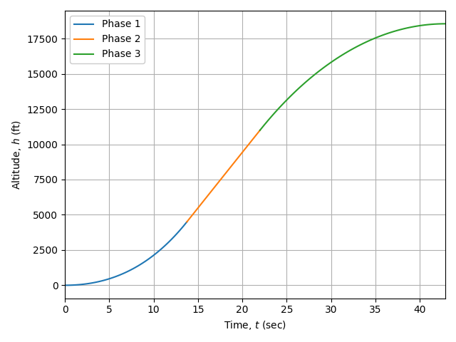
# altitude
plt.figure(2)
ax = plt.axes()
line = []
for p in range(3):
line1 = ax.plot(time[p], state[p][0])
line.append(line1)
plt.ylabel("Altitude, $h$ (ft)")
# velocity
plt.figure(3)
ax = plt.axes()
line = []
for p in range(3):
line1 = ax.plot(time[p], state[p][1])
line.append(line1)
plt.ylabel("Velocity, $v$ (ft/s)")
# mass
plt.figure(4)
ax = plt.axes()
line = []
for p in range(3):
line1 = ax.plot(time[p], state[p][2])
line.append(line1)
plt.ylabel("Mass, $m$ (slugs)")
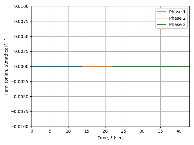
# hamiltonian
plt.figure(5)
ax = plt.axes()
line = []
for p in range(3):
hamiltonian = sum(dynamics[p][i] * costate[p][i] for i in range(3))
line1 = ax.plot(time_c[p], hamiltonian)
line.append(line1)
plt.ylim([-0.01, 0.01])
plt.ylabel(r"Hamiltonian, $\mathcal{H}")
for i in range(1, 6):
plt.figure(i)
plt.legend(("Phase 1", "Phase 2", "Phase 3"), framealpha=1.0)
plt.xlabel("Time, $t$ (sec)")
plt.xlim([t0, tf])
plt.tight_layout()
plt.grid()
def main() -> None:
"""Demonstrate the solution to the Goddard Rocket Problem (3 phases)."""
problem = setup()
solution = problem.solve()
plot_solution(solution)
plt.show()
if __name__ == "__main__":
main()
Text Output
******************************************************************************
This program contains Ipopt, a library for large-scale nonlinear optimization.
 Ipopt is released as open source code under the Eclipse Public License (EPL).
         For more information visit https://github.com/coin-or/Ipopt
******************************************************************************

Total number of variables............................:     1001
                     variables with only lower bounds:        0
                variables with lower and upper bounds:      906
                     variables with only upper bounds:        0
Total number of equality constraints.................:      999
Total number of inequality constraints...............:        3
        inequality constraints with only lower bounds:        3
   inequality constraints with lower and upper bounds:        0
        inequality constraints with only upper bounds:        0


Number of Iterations....: 31

                                   (scaled)                 (unscaled)
Objective...............:  -1.8550871863824483e+04    1.8550871863824483e+04
Dual infeasibility......:   1.2732925824820995e-11    1.2732925824820995e-11
Constraint violation....:   1.2123564374633133e-09    1.2123564374633133e-09
Variable bound violation:   2.2204460492503131e-16    2.2204460492503131e-16
Complementarity.........:   9.9927165098521219e-16    9.9927165098521219e-16
Overall NLP error.......:   1.2123564374633133e-09    1.2123564374633133e-09


Number of objective function evaluations             = 34
Number of objective gradient evaluations             = 32
Number of equality constraint evaluations            = 34
Number of inequality constraint evaluations          = 34
Number of equality constraint Jacobian evaluations   = 32
Number of inequality constraint Jacobian evaluations = 32
Number of Lagrangian Hessian evaluations             = 31
Total seconds in IPOPT (w/o function evaluations)    =      0.780
Total seconds in NLP function evaluations            =      0.295

EXIT: Solved To Acceptable Level.
Plots
Thrust

Altitude
Velocity

Mass

Hamiltonian