Dynamic Soaring
For a description of the dynamic soaring problem, see the dynamic soaring JupyterLab notebook documentation for this problem.
The python script in this example can be executed from the command line with:
$ python -m yapss.examples.dynamic_soaring
Functions
YAPSS solution of the dynamic soaring optimal control problem.
Code
"""
YAPSS solution of the dynamic soaring optimal control problem.
"""
__all__ = ["main", "plot_solution", "setup"]
from typing import TYPE_CHECKING
# third party imports
import matplotlib.pyplot as plt
# package imports
import numpy as np
from mpl_toolkits.mplot3d import Axes3D
from yapss import ContinuousArg, DiscreteArg, ObjectiveArg, Problem, Solution
from yapss.math import cos, sin
if TYPE_CHECKING:
from numpy.typing import NDArray
def setup() -> Problem:
"""Set up the dynamic soaring optimal control problem.
Returns
-------
Problem
The dynamic soaring optimal control problem.
"""
# initialize the optimal control problem
ocp = Problem(name="Dynamic Soaring", nx=[6], nu=[2], nh=[1], ns=1, nd=3)
# problem callback functions
def objective(arg: ObjectiveArg) -> None:
"""Dynamic soaring objective function."""
arg.objective = arg.parameter[0]
def continuous(arg: ContinuousArg) -> None:
"""Dynamic soaring continuous function."""
auxdata = arg.auxdata
_, _, h, v, gamma, psi = arg.phase[0].state
cl, phi = arg.phase[0].control
beta = arg.parameter[0]
w = auxdata.m * auxdata.g0
q = auxdata.rho0 * v**2 / 2
cd = auxdata.cd0 + auxdata.k * cl**2
lift = q * auxdata.s * cl
drag = q * auxdata.s * cd
wx = beta * h + auxdata.w0
cos_gamma = cos(gamma)
sin_gamma = sin(gamma)
cos_psi = cos(psi)
sin_psi = sin(psi)
cos_phi = cos(phi)
sin_phi = sin(phi)
x_dot = v * cos_gamma * sin_psi + wx
y_dot = v * cos_gamma * cos_psi
h_dot = v * sin_gamma
wx_dot = beta * h_dot
v_dot = -drag / auxdata.m - auxdata.g0 * sin_gamma - wx_dot * cos_gamma * sin_psi
gamma_dot = lift * cos_phi - w * cos_gamma + auxdata.m * wx_dot * sin_gamma * sin_psi
gamma_dot /= auxdata.m * v
psi_dot = (lift * sin_phi - auxdata.m * wx_dot * cos_psi) / (auxdata.m * v * cos_gamma)
arg.phase[0].dynamics[:] = x_dot, y_dot, h_dot, v_dot, gamma_dot, psi_dot
arg.phase[0].dynamics[:] = x_dot, y_dot, h_dot, v_dot, gamma_dot, psi_dot
arg.phase[0].path[:] = ((0.5 * auxdata.rho0 * auxdata.s / w) * cl * v**2,)
def discrete(arg: DiscreteArg) -> None:
"""Dynamic soaring discrete function."""
x0 = arg.phase[0].initial_state
xf = arg.phase[0].final_state
arg.discrete = xf[3:] - x0[3:]
# user callback functions
ocp.functions.objective = objective
ocp.functions.continuous = continuous
ocp.functions.discrete = discrete
# define the auxiliary data
auxdata = ocp.auxdata
auxdata.w0 = 0
auxdata.g0 = 32.2
auxdata.cd0 = 0.00873
auxdata.rho0 = 0.002378
auxdata.m = 5.6
auxdata.s = 45.09703
auxdata.k = 0.045
auxdata.cl_max = 1.5
# set bounds
bounds = ocp.bounds.phase[0]
bounds.initial_time.lower = 0
bounds.initial_time.upper = 0
bounds.final_time.lower = 10
bounds.final_time.upper = 30
bounds.initial_state.lower[:3] = bounds.initial_state.upper[:3] = 0, 0, 0
bounds.final_state.lower[:3] = bounds.final_state.upper[:3] = 0, 0, 0
bounds.state.lower = -1500, -1000, 0, 10, np.radians(-75), np.radians(-225)
bounds.state.upper = +1500, +1000, 1000, 350, np.radians(75), np.radians(225)
bounds.control.lower = 0, np.radians(-75)
bounds.control.upper = auxdata.cl_max, np.radians(75)
bounds.path.lower = (-2,)
bounds.path.upper = (5,)
ocp.bounds.discrete.lower = ocp.bounds.discrete.upper = 0, 0, np.radians(360)
# scaling to improve convergence rate
scale = ocp.scale
scale.objective = 0.1
scale.parameter = [0.1]
scale.discrete = [200.0, 200.0, 200.0]
phase = scale.phase[0]
phase.dynamics = phase.state = 1000.0, 1000.0, 1000.0, 200.0, 1.0, 6.0
phase.control = 1.0, 1.0
phase.time = 30.0
phase.path = [7.0]
# generate guess
pi = np.pi
tf = 24
one: NDArray[np.float64] = np.ones(50, dtype=float)
t: NDArray[np.float64] = np.linspace(0, tf, num=50, dtype=float)
y = -200 * np.sin(2 * pi * t / tf)
x = 600 * (np.cos(2 * pi * t / tf) - 1)
h = -0.7 * x
v = 150 * one
gamma = 0 * one
psi = np.radians(t / tf * 360)
cl = 0.5 * one
phi = np.radians(45) * one
ocp.guess.phase[0].time = t
ocp.guess.phase[0].state = x, y, h, v, gamma, psi
ocp.guess.phase[0].control = cl, phi
ocp.guess.parameter = (0.08,)
# define a fairly dense mesh to capture discontinuity in derivatives
m, n = 50, 6
ocp.mesh.phase[0].collocation_points = m * (n,)
ocp.mesh.phase[0].fraction = m * (1.0 / m,)
ocp.spectral_method = "lgl"
# define derivatives
ocp.derivatives.method = "auto"
ocp.derivatives.order = "second"
# ipopt options
ocp.ipopt_options.max_iter = 500
ocp.ipopt_options.print_level = 3
return ocp
def plot_solution(solution: Solution) -> None:
"""Plot the solution to the dynamic soaring optimal control problem.
Parameters
----------
solution : Solution
The solution to the dynamic soaring optimal control problem.
"""
# extract information from solution
auxdata = solution.problem.auxdata
t = solution.phase[0].time
tc = solution.phase[0].time_c
x, y, h, v, gamma, psi = solution.phase[0].state
cl, phi = solution.phase[0].control
hamiltonian = solution.phase[0].hamiltonian
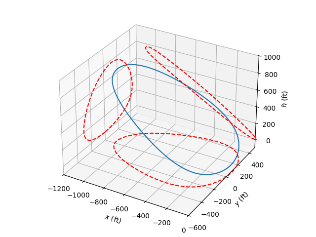
# figure 1: plot the path in 3D
plt.figure(1)
ax: Axes3D = plt.axes(projection=Axes3D.name)
ax.plot3D(x, y, h)
ax.plot3D(0 * x - 1200, y, h, "r--")
ax.plot3D(x, 0 * y + 500, h, "r--")
ax.plot3D(x, y, 0 * h - 100, "r--")
ax.set_xlim([-1200, 0])
ax.set_ylim([-600, 500])
ax.set_zlim([-100, 1000])
ax.set_xlabel(r"$x$ (ft)")
ax.set_ylabel(r"$y$ (ft)")
ax.set_zlabel(r"$h$ (ft)")
plt.tight_layout()
# figure 2: Lift coefficient
plt.figure(2)
limit = 5 * (auxdata.m * auxdata.g0) / (0.5 * auxdata.rho0 * auxdata.s * v**2)
plt.plot(t, limit, "r--")
plt.plot(tc, cl)
plt.ylim([0, 1])
legend = plt.legend(["Load factor limit", "Lift coefficient, $C_{L}$"])
legend.get_frame().set_facecolor("white")
legend.get_frame().set_alpha(1)
legend.get_frame().set_linewidth(0)
plt.ylabel(r"Lift coefficient, $C_L$")
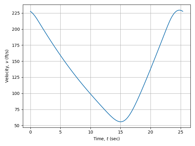
# figure 3: velocity
plt.figure(3)
plt.plot(t, v)
plt.ylabel(r"Velocity, $v$ (ft/s)")
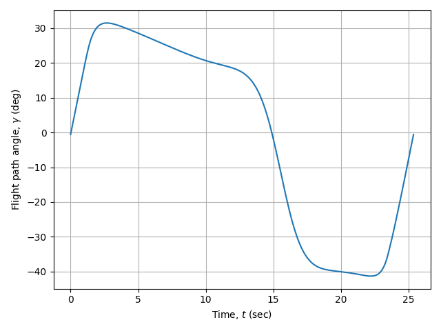
# figure 4: gamma
plt.figure(4)
plt.plot(t, np.rad2deg(gamma))
plt.ylabel(r"Flight path angle, $\gamma$ (deg)")
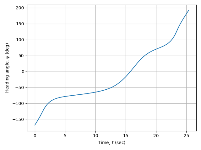
# figure 5: psi
plt.figure(5)
plt.plot(t, np.rad2deg(psi))
plt.ylabel(r"Heading angle, $\psi$ (deg)")
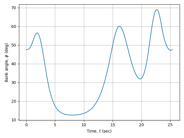
# figure 6: bank angle
plt.figure(6)
plt.plot(tc, np.rad2deg(phi))
plt.ylabel(r"Bank angle, $\phi$ (deg)")
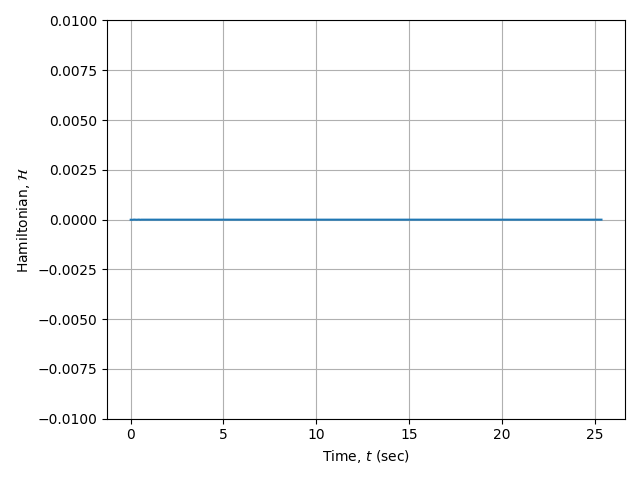
# figure 7: Hamiltonian
plt.figure(7)
plt.plot(tc, hamiltonian)
plt.ylabel(r"Hamiltonian, $\mathcal{H}$")
plt.ylim([-0.01, 0.01])
for i in range(2, 8):
plt.figure(i)
plt.xlabel(r"Time, $t$ (sec)")
plt.tight_layout()
plt.grid()
def main() -> None:
"""Demonstrate the solution to the dynamic soaring optimal control problem."""
problem = setup()
solution = problem.solve()
plot_solution(solution)
plt.show()
if __name__ == "__main__":
main()
Text Output
******************************************************************************
This program contains Ipopt, a library for large-scale nonlinear optimization.
 Ipopt is released as open source code under the Eclipse Public License (EPL).
         For more information visit https://github.com/coin-or/Ipopt
******************************************************************************

Total number of variables............................:     2304
                     variables with only lower bounds:        0
                variables with lower and upper bounds:     2003
                     variables with only upper bounds:        0
Total number of equality constraints.................:     1803
Total number of inequality constraints...............:      252
        inequality constraints with only lower bounds:        1
   inequality constraints with lower and upper bounds:      251
        inequality constraints with only upper bounds:        0


Number of Iterations....: 32

                                   (scaled)                 (unscaled)
Objective...............:   6.3586558207092936e-01    6.3586558207092941e-02
Dual infeasibility......:   1.8260011056998176e-13    1.8260011056998176e-14
Constraint violation....:   9.3851176830028749e-11    4.7944936909516400e-10
Variable bound violation:   0.0000000000000000e+00    0.0000000000000000e+00
Complementarity.........:   1.0051386917517832e-11    1.0051386917517832e-12
Overall NLP error.......:   9.3851176830028749e-11    4.7944936909516400e-10


Number of objective function evaluations             = 33
Number of objective gradient evaluations             = 33
Number of equality constraint evaluations            = 33
Number of inequality constraint evaluations          = 33
Number of equality constraint Jacobian evaluations   = 33
Number of inequality constraint Jacobian evaluations = 33
Number of Lagrangian Hessian evaluations             = 32
Total seconds in IPOPT (w/o function evaluations)    =      2.471
Total seconds in NLP function evaluations            =      0.630

EXIT: Optimal Solution Found.
Plots
Optimal Trajectory
Velocity
Flight Path Angle
Heading Angle
Lift Coefficient

Bank Angle
Hamiltonian