Newton’s Minimal Resistance Problem
For a solution to the Newton’s minimal resistance problem using a Python script instead of a notebook, see the Python script documentation.
Problem Description
Newton’s Minimal Resistance Problem is the first known calculus of variations problem, published in Isaac Newton’s Principia Mathematica in 1687 [1]. The problem is to find the convex solid of revolution (a nose cone) that has the lowest resistance (drag) when it moves through a rarefied gas along the axis of symmetry. In Newton’s model, gas particles do not interact with each other, and bounce off the nose cone elastically with no loss. The nose cone is assumed to be convex (and axisymmetric) so that there are no additional collisions after the first. For a modern treatment of Newton’s problem, including the assumption of convexity and axisymmetry, see the paper by Buttazzo and Kawohl [2]. The convexity assumption is stronger than required to assure that each particle experiences only a single collision, but relaxing the convexity and axisymmetry assumptions while ensuring that each particle experiences only a single collision is quite complicated. See for example the paper by Compte and Lachand-Robert [3]. For this example, we’ll keep Newton’s simpler assumptions.
Consider first the drag on a right circular cylinder with radius \(R\). A gas particle with velocity \(v\) relative to the body will bounce elastically off the circular end with velocity \(v\) in the opposite direction. For a particle with mass \(m\), the net impulse on the cylinder will then be the net change in momentum of the particle, \(2mv\). For the rarefied gas, the drag is similarly twice the momentum flux striking the end of the cylinder, \(D=2 \rho v^2 \pi R^2\). The drag coefficient is then
For a more general convex, axisymmetric nose cone, we define \(\theta\) at each point on the surface of the cone as the angle between the axis of symmetry of the nose cone and the normal to the surface. Then each particle that strikes the surface rebounds at angle angle \(2 \theta\) away from the axis of symmetry. As a result, the local drag coefficient is
where \(\Delta D\) is the drag due to forces on a small patch of the surface, and \(\Delta A\) is the area of the small patch of the surface projected onto a plane normal to the axis of symmetry.
For a nose cone of radius \(R\), the total drag coefficient is then
Take the height of the nose cone at each radial station to be \(y(r)\). Using a little trigonometry, we can express \((\cos\theta(r))^2\) as
where
Therefore, the cost objective to be minimized is
Note that for a blunt nose cone (cylinder) \(J=4\).
(Most treatments of Newton’s minimal resistance problem normalize the drag by the drag of a right circular cylinder rather than using the more modern drag coefficient, and hence our objective is a factor of 4 larger.)
There are constraints on the shape of the nose cone. First, in the limit of very long, slender bodies, the drag is zero, and so we must limit the height of the nose cone by, say,
Second, the convexity of the nose cone requires that
Then the state for the problem is \(\boldsymbol{x} = [y(r),y^{\prime}(r)]\)s, and the control is \(u(r)=y^{\prime\prime}\). Then dynamics then are given by
Therefore, the constraints become
Finally, note that the independent variable is not time, but rather the radius \(r\).
YAPSS Solution
First, we import the required Python packages:
[1]:
# third party imports
import matplotlib.pyplot as plt
import numpy as np

# package imports
from yapss import Problem, Solution
Instantiate the optimal control problem with two states, one control input, and one integral:
[2]:
# instantiate the problem
problem = Problem(
    name="Newton's minimal resistance problem",
    nx=[2],
    nu=[1],
    nq=[1],
)
Define the objective and continuous callback functions:
[3]:
# callback functions


def objective(arg):
    """Objective function for Newton's minimal resistance problem."""
    arg.objective = arg.phase[0].integral[0]


def continuous(arg):
    """Newton's minimal resistance problem dynamics and cost integrand."""
    _, yp = arg.phase[0].state
    (u,) = arg.phase[0].control
    r = arg.phase[0].time
    arg.phase[0].dynamics[:] = yp, u
    arg.phase[0].integrand[:] = (8 * r / (1 + yp**2),)


problem.functions.objective = objective
problem.functions.continuous = continuous
Define a function to set up the problem. For most of the JupyterLab notebook examples, we don’t use a setup function. But we do it here because some of the settings (bounds, initial guess) depend on a parameter that we want to vary.
[4]:
def setup(y_max: float = 1.0) -> Problem:
    """Set up Newton's minimal resistance problem as an optimal control problem."""
    ocp = Problem(
        name="Newton's minimal resistance problem",
        nx=[2],
        nu=[1],
        nq=[1],
    )

    # functions
    ocp.functions.objective = objective
    ocp.functions.continuous = continuous

    # bounds
    bounds = ocp.bounds.phase[0]
    bounds.initial_time.lower = bounds.initial_time.upper = 0.0
    bounds.final_time.lower = bounds.final_time.upper = 1.0
    bounds.state.lower[0] = 0
    bounds.state.upper = y_max, 0
    bounds.control.upper = (0,)

    # guess
    phase = ocp.guess.phase[0]
    phase.time = [0.0, 1.0]
    phase.state = [[y_max, 0.0], [-y_max, -y_max]]
    phase.control = [[0.0, 0.0]]

    # solver settings
    ocp.derivatives.order = "second"
    ocp.derivatives.method = "auto"
    ocp.spectral_method = "lgl"

    # ipopt settings
    ocp.ipopt_options.print_level = 3
    ocp.ipopt_options.sb = "yes"

    return ocp
Now set up the problem for a particular maximum value of \(y\) and solve:
[5]:
# nosecone height of 1.0
problem = setup(y_max=1)
solution = problem.solve()
Total number of variables............................:      294
                     variables with only lower bounds:        0
                variables with lower and upper bounds:       91
                     variables with only upper bounds:      182
Total number of equality constraints.................:      201
Total number of inequality constraints...............:        1
        inequality constraints with only lower bounds:        1
   inequality constraints with lower and upper bounds:        0
        inequality constraints with only upper bounds:        0


Number of Iterations....: 59

                                   (scaled)                 (unscaled)
Objective...............:   1.5033522844315192e+00    1.5033522844315192e+00
Dual infeasibility......:   3.0936063001488095e-09    3.0936063001488095e-09
Constraint violation....:   2.2644626174184168e-09    2.2644626174184168e-09
Variable bound violation:   9.0877322414097458e-09    9.0877322414097458e-09
Complementarity.........:   5.2160264124442990e-09    5.2160264124442990e-09
Overall NLP error.......:   5.2160264124442990e-09    5.2160264124442990e-09


Number of objective function evaluations             = 60
Number of objective gradient evaluations             = 60
Number of equality constraint evaluations            = 60
Number of inequality constraint evaluations          = 60
Number of equality constraint Jacobian evaluations   = 60
Number of inequality constraint Jacobian evaluations = 60
Number of Lagrangian Hessian evaluations             = 59
Total seconds in IPOPT (w/o function evaluations)    =      0.301
Total seconds in NLP function evaluations            =      0.118

EXIT: Optimal Solution Found.
[6]:
print(f"Minimum drag solution has CD = {solution.objective:.5f}")
Minimum drag solution has CD = 1.50335
We’re going to plot multiple solutions, so define a plot function, and go ahead and plot:
[7]:
def plot_solution(solution: Solution) -> None:
    """Plot solution."""
    # plot style information
    linewidth = 2
    plt.rc("font", size=14)
    plt.rc("font", family="sans-serif")

    # extract information from solution
    r = solution.phase[0].time
    y, _ = solution.phase[0].state
    r = np.concatenate((-r[-1::-1], r))
    y = np.concatenate((y[-1::-1], y))

    # plot
    h = plt.plot(r, y, "r", linewidth=linewidth)
    plt.axis("equal")
    plt.xlim([-1, 1])
    plt.ylim([-0.1, 2.1])
    plt.xlabel("Radius, $r/R$")
    plt.ylabel("Height, $y/R$")
    plt.tight_layout()
    return h


# plot solution for nosecone height = 1.0
plot_solution(solution)
plt.ylim([-0.1, 1.1])
plt.gca().get_figure().set_figheight(3)
Ignoring fixed x limits to fulfill fixed data aspect with adjustable data limits.
Ignoring fixed x limits to fulfill fixed data aspect with adjustable data limits.

If we zoom in on one of the corners of the solution, we see that what we expect would be a sharp corner is in fact quite rounded:
[8]:
# zoom in on solution to see detail at corner
h = plot_solution(solution)
h[0].set_linewidth(1)
h[0].set_marker("o")
plt.ylim([0.975, 1.025])
plt.xlim([0.28, 0.36])
plt.gca().get_figure().set_figheight(3)
Ignoring fixed x limits to fulfill fixed data aspect with adjustable data limits.
Ignoring fixed x limits to fulfill fixed data aspect with adjustable data limits.
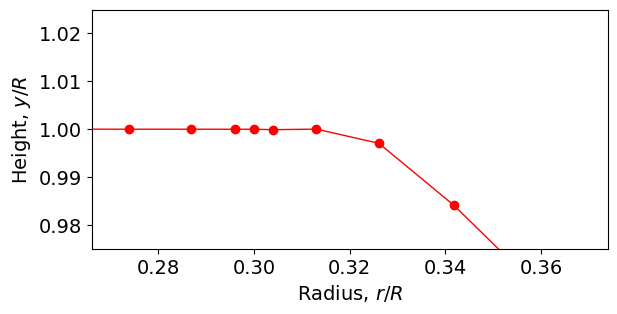
The reason for this is that the polynomials that represent the height \(y(r)\) can’t represent a sharp corner well. To fix this, we’ll assume that the height is constant below some radius \(r_0\), so that
The radius \(r_0\) becomes our new initial time (instead of 0). To get the right drag, we have to add a new term to the objective which accounts for the integral for \(0 \le r \le r_0\), which is
when \(R=1\) as in our formulation. We must also allow the “initial time” to range over \(0\le r_0 \le 1\).
[9]:
# modify objective for new problem formulation


def objective2(arg):
    """Improved objective function for Newton's minimal resistance problem."""
    arg.objective = arg.phase[0].integral[0] + 4 * arg.phase[0].initial_time ** 2


def setup2(y_max: float = 1.0) -> Problem:
    """Modify original setup to account for the new objective and boundary conditions."""
    ocp = setup(y_max)
    ocp.functions.objective = objective2
    ocp.bounds.phase[0].initial_time.upper = 1.0
    return ocp
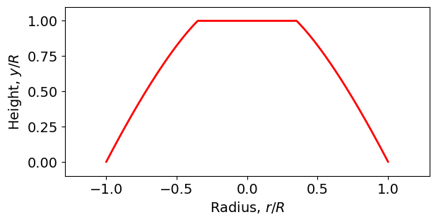
If we now look at the solution, we have a much better result.
[10]:
# solve new problem formulation with nosecone height = 1.0
problem = setup2(y_max=1)
solution = problem.solve()
Total number of variables............................:      295
                     variables with only lower bounds:        0
                variables with lower and upper bounds:       92
                     variables with only upper bounds:      182
Total number of equality constraints.................:      201
Total number of inequality constraints...............:        1
        inequality constraints with only lower bounds:        1
   inequality constraints with lower and upper bounds:        0
        inequality constraints with only upper bounds:        0


Number of Iterations....: 14

                                   (scaled)                 (unscaled)
Objective...............:   1.4992639210690413e+00    1.4992639210690413e+00
Dual infeasibility......:   6.5203275837075868e-09    6.5203275837075868e-09
Constraint violation....:   4.2988782533726067e-09    4.2988782533726067e-09
Variable bound violation:   9.9813749993299214e-09    9.9813749993299214e-09
Complementarity.........:   1.1308533134617289e-09    1.1308533134617289e-09
Overall NLP error.......:   6.5203275837075868e-09    6.5203275837075868e-09


Number of objective function evaluations             = 16
Number of objective gradient evaluations             = 15
Number of equality constraint evaluations            = 16
Number of inequality constraint evaluations          = 16
Number of equality constraint Jacobian evaluations   = 15
Number of inequality constraint Jacobian evaluations = 15
Number of Lagrangian Hessian evaluations             = 14
Total seconds in IPOPT (w/o function evaluations)    =      0.039
Total seconds in NLP function evaluations            =      0.026

EXIT: Optimal Solution Found.
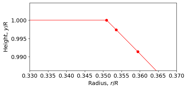
[11]:
# plot solution with new problem formulation
plt.figure()
plot_solution(solution)
plt.ylim([-0.1, 1.1])
plt.gca().get_figure().set_figheight(3)

plt.figure()
h = plot_solution(solution)
h[0].set_linewidth(1)
h[0].set_marker("o")
plt.ylim([0.99, 1.001])
plt.xlim([0.33, 0.37])
plt.gca().get_figure().set_figheight(3)
Ignoring fixed x limits to fulfill fixed data aspect with adjustable data limits.
Ignoring fixed x limits to fulfill fixed data aspect with adjustable data limits.
Ignoring fixed x limits to fulfill fixed data aspect with adjustable data limits.
Ignoring fixed y limits to fulfill fixed data aspect with adjustable data limits.
Optimal nose cones for three different aspect ratios, \(y_{\text{max}}/R=0.5\), \(y_{\text{max}}/R=1.0\), and \(y_{\text{max}}/R=2.0\), using improved objective function.
[12]:
# plot solution for various nosecone heights
plt.figure(figsize=(6.4, 6.4))
for y_max in (0.5, 1.0, 2.0):
    problem = setup2(y_max=y_max)
    problem.ipopt_options.print_level = 0
    solution = problem.solve()
    plot_solution(solution)
    print(f"{y_max = }, Coefficient of drag = {solution.objective:0.10f}")

print("\n")
Ignoring fixed x limits to fulfill fixed data aspect with adjustable data limits.
Ignoring fixed x limits to fulfill fixed data aspect with adjustable data limits.
Ignoring fixed x limits to fulfill fixed data aspect with adjustable data limits.
y_max = 0.5, Coefficient of drag = 2.4300290384
y_max = 1.0, Coefficient of drag = 1.4992639211
y_max = 2.0, Coefficient of drag = 0.6417019938
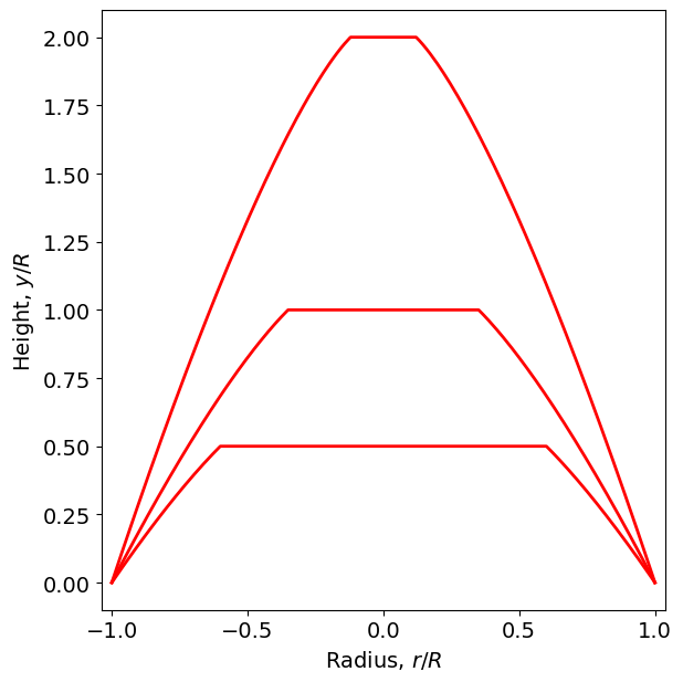
It’s straightforward to show that the optimal drag coefficient depends on the nondimensional ratio \(y_{\text{max}}/R\), so without loss of generality the cases run here are for \(R=1\). Data for three cases, \(y_{\text{max}}/R=0.5\), 1.0, and 2.0, are shown below. In the table we also show the limiting cases \(y_{\text{max}}/R=0\) and \(y_{\text{max}}/R=\infty\).