Delta III Launch Vehicle Ascent Problem
In his PhD thesis, Benson [1] presents the example of the optimization of the Delta III launch vehicle to minimize fuel used to achieve a specific orbit. Rao et al. [2] and Patterson and Rao [3] used the same example (with only very slightly modified numerical parameters) as an example in their papers describing the GPOPS and GPOPS-II algorithms. The problem is also described in some detail by Betts [4].
For a solution to the Delta III launch vehicle ascent problem using a Python script instead of a notebook, see the corresponding Python script documentation.
Problem Definition
Quantity |
Symbol |
Solid rocket boosters |
Stage 1 |
Stage 2 |
|---|---|---|---|---|
Total mass (kg) |
\(\pi_i\) |
19290 |
104380 |
19300 |
Propellant mass (kg) |
\(\rho_i\) |
17010 |
95550 |
16820 |
Structure Mass (kg) |
\(\varphi_i\) |
2280 |
8830 |
2480 |
Engine thrust (N) |
\(T_i\) |
628500 |
1083100 |
110094 |
Specific impulse (s) |
\(\mathcal{I_i}\) |
283.33364 |
301.68776 |
467.21311 |
Number of engines |
\(N\) |
9 |
1 |
1 |
Burn time (s) |
\(\tau_i\) |
75.2 |
261 |
700 (max) |
Dynamics. The dynamics are described in an Earth-centered inertial (ECI) coordinate system. The seven states are the three elements of the position vector \(\mathbf{r}\), the three elements of the inertial velocity vector \(\mathbf{v}\), and the vehicle mass \(m\). The dynamics for each stage are given by
where \(\mu\) is the gravitational parameter for Earth, \(T\) is the thrust, \(\mathbf{u}\) is the control input, \(\mathbf{D}\) is the drag force, and \(\xi\) is the propellant burn rate. The control vector defines the thrust direction, and so is a 3-vector with the constraint
An additional constraint is that
where \(R_{E}\) is the radius of the earth. That is, that the vehicle always has nonnegative altitude. The constraints are expressed as path constraints in the continuous callback function.
Aerodynamics. The drag force is always in the opposite direction to the relative velocity of the vehicle through the atmosphere, and so
where
Here \(\boldsymbol{\Omega} = (0, 0, \omega_E)\) is the angular velocity of the earth. The density of the atmosphere is assumed to be exponential
where \(\rho_{0}\) is the sea-level density of the atmosphere, and \(H\) is the scale height of the atmosphere.
Orbital Element |
Symbol |
Value at final time |
|---|---|---|
Semimajor axis |
\(a_f\) |
\(2.4361140\times10^7\) m |
Eccentricity |
\(e_f\) |
\(0.7308\) |
Inclination |
\(i_f\) |
\(28.5^{\circ}\) |
Longitude of the ascending node |
\(\Omega_f\) |
\(269.8^{\circ}\) |
Argument of the periapsis |
\(\omega_f\) |
\(130.5^{\circ}\) |
Constant |
Symbol |
Value |
|---|---|---|
Payload Mass |
\(\pi_\text{p}\) |
\(4164 \text{ kg}\) |
Aerodynamic reference area |
\(S\) |
\(4 \pi \text{ m}^{2}\) |
Coefficient of drag |
\(C_{D}\) |
\(0.5\) |
Atmospheric density at sea level |
\(\rho_{0}\) |
\(1.225 \text{ kg/m}^{3}\) |
Atmospheric density scale height |
\(H\) |
\(7200 \text{ m}\) |
Time at end of first phase |
\(t_{1}\) |
\(75.2 \text{ s}\) |
Time at end of second phase |
\(t_{2}\) |
\(150.4 \text{ s}\) |
Time at end of third phase |
\(t_{3}\) |
\(261 \text{ s}\) |
Radius of earth |
\(R_E\) |
\(6378145 \text{ m}\) |
Earth rotation rate |
\(\Omega\) |
\(7.29211585 \times 10^{-5} \text{ rad}/\text{s}\) |
Earth gravitational parameter |
\(\mu\) |
\(3.986012 \times 10^{14} \text { m}^3/\text{s}^2.\) |
Standard gravity |
\(g_{0}\) |
\(9.80665 \text{ m} / \text{s}^{2}\) |
YAPSS Solution
Problem Instantation
First import needed packages and instantiate problem:
[1]:
# third party imports
import numpy as np
from matplotlib import pyplot as plt

# package imports
from yapss import Problem
from yapss.math import cos, pi, sin, sqrt

problem = Problem(
    name="Delta III Ascent Trajectory Optimization",
    nx=[7, 7, 7, 7],
    nu=[3, 3, 3, 3],
    nh=[2, 2, 2, 2],
    nd=23,
)
Constants
The problem has lots of constants that must be defined:
[2]:
# Dynamic Model Parameters
mu = 3.986012e14  # earth gravity parameter
R_e = 6378145.0  # earth radius
g0 = 9.80665  # sea-level gravity
h0 = 7200.0  # atmospheric density scale height
rho0 = 1.225  # sea-level air density
omega_e = 7.29211585e-5  # earth rotation rate
CD = 0.5  # coefficient of drag
S = 4 * pi  # aerodynamic reference area
psi_l = 28.5 * pi / 180.0  # latitude of launch site
q_max = 100000.0  # dynamic pressure bound

# Vehicle parameters
# srb, first stage, second stage, payload masses (kg)
pi_s, pi_1, pi_2, pi_p = 19290.0, 104380.0, 19300.0, 4164.0

# propellant masses (kg)
rho_s, rho_1, rho_2 = 17010.0, 95550.0, 16820.0

# dry masses
phi_s = pi_s - rho_s
phi_1 = pi_1 - rho_1
phi_2 = pi_2 - rho_2

# srb, first stage, second stage thrust (N)
Ts, T1, T2 = 628500.0, 1083100.0, 110094.0

# burn times
tau_s, tau_1, tau_2 = 75.2, 261.0, 700.0

# initial total mass of vehicle
m_total = 9 * pi_s + pi_1 + pi_2 + pi_p

# initial time for each phase
t0, t1, t2, t3 = 0.0, 75.2, 150.4, 261.0

# max final time
t4_max = t3 + tau_2

# srb, first stage, second stage specific impulse (sec)
Is = Ts * tau_s / (rho_s * g0)
I1 = T1 * tau_1 / (rho_1 * g0)
I2 = T2 * tau_2 / (rho_2 * g0)

# orbital parameters for desired orbit
a_f, e_f, i_f, Omega_f, omega_f = 24361140, 0.7308, 28.5, 269.8, 130.5

# initial position
r0_vec = R_e * cos(psi_l), 0.0, R_e * sin(psi_l)

# initial and final masses for the 4 phases
mi_0 = 9 * pi_s + pi_1 + pi_2 + pi_p
mf_0 = mi_0 - 6 * rho_s - tau_s / tau_1 * rho_1

mi_1 = mf_0 - 6 * phi_s
mf_1 = mi_1 - 3 * rho_s - tau_s / tau_1 * rho_1

mi_2 = mf_1 - 3 * phi_s
mf_2 = mi_2 - (1 - 2 * tau_s / tau_1) * rho_1

mi_3 = mf_2 - phi_1
Callback Functions
Before defining the callback functions, we need some helper functions to compute cross products, magnitudes, and dot products for vectors:
[3]:
def cross(x1, x2):
    """Vector cross product."""
    x3 = [0, 0, 0]
    x3[0] = x1[1] * x2[2] - x1[2] * x2[1]
    x3[1] = x1[2] * x2[0] - x1[0] * x2[2]
    x3[2] = x1[0] * x2[1] - x1[1] * x2[0]
    return x3


def mag(x):
    """Vector magnitude."""
    return (sum(xi**2 for xi in x) + 1e-100) ** 0.5


def dot(x1, x2):
    """Vector _dot product."""
    return sum(x1[i] * x2[i] for i in range(3))
Functions that convert back and forth between between orbital elements and position, velocity vectors:
[4]:
def oe_to_rv(a, e, i, Omega, omega, nu, mu_):
    """Convert orbital elements to cartesian position and velocity.

    Parameters
    ----------
        a: semimajor axis
        e: eccentricity
        i: inclination
        Omega: longitude of the ascending node (degrees)
        omega: argument of the periapsis (degrees)
        nu: true anomaly
        mu: Gravitational parameter

    Returns
    -------
        Tuple[ArrayLike]: Inertial position and velocity vectors
    """
    # pylint: disable=too-many-arguments
    p = a * (1 - e**2)
    r = p / (1 + e * cos(nu))
    r_vec = np.array([r * cos(nu), r * sin(nu), 0])
    v_vec = sqrt(mu_ / p) * np.array([-sin(nu), e + cos(nu), 0])
    deg_to_rad = pi / 180
    c_O = cos(deg_to_rad * Omega)
    s_O = sin(deg_to_rad * Omega)
    c_o = cos(deg_to_rad * omega)
    s_o = sin(deg_to_rad * omega)
    c_i = cos(deg_to_rad * i)
    s_i = sin(deg_to_rad * i)
    R = [
        [c_O * c_o - s_O * s_o * c_i, -c_O * s_o - s_O * c_o * c_i, +s_O * s_i],
        [s_O * c_o + c_O * s_o * c_i, -s_O * s_o + c_O * c_o * c_i, -c_O * s_i],
        [s_o * s_i, c_o * s_i, c_i],
    ]
    R = np.array(R)
    r_vec = R @ r_vec
    v_vec = R @ v_vec
    return r_vec, v_vec


def rv_to_oe(r_vec, v_vec):
    r"""Compute orbital elements from position and velocity vectors.

    The function is a simplified calculation of (some of) the orbital elements, without
    checking for special cases.

    Parameters
    ----------
        r_vec : 3-dimensional position vector
        v_vec : 3-dimensional velocity vector

    Returns
    -------
    Tuple[ArrayLike]
        Five of the six orbital elements: semimajor axis, eccentricity, inclination,
        longitude of the ascending node, argument of the periapsis
    """
    # http://www.aerospacengineering.net/determining-orbital-elements/
    r = mag(r_vec)
    v = mag(v_vec)
    h_vec = cross(r_vec, v_vec)
    h = mag(h_vec)
    n_vec = cross([0, 0, 1], h_vec)
    n = mag(n_vec)
    e0 = ((v**2 - mu / r) * r_vec[0] - dot(r_vec, v_vec) * v_vec[0]) / mu
    e1 = ((v**2 - mu / r) * r_vec[1] - dot(r_vec, v_vec) * v_vec[1]) / mu
    e2 = ((v**2 - mu / r) * r_vec[2] - dot(r_vec, v_vec) * v_vec[2]) / mu
    e_vec = (e0, e1, e2)
    e = mag(e_vec)
    a = 1 / (2 / r - v**2 / mu)
    i = np.arccos(h_vec[2] / h) * 180 / pi
    Omega = 360 - np.arccos(n_vec[0] / n) * 180 / pi
    omega = np.arccos(dot(n_vec, e_vec) / (n * e)) * 180 / pi
    return a, e, i, Omega, omega
The callback functions:
[5]:
def objective(arg):
    """Calculate Delta III ascent trajectory optimization problem objective."""
    # maximize the final mass
    arg.objective = -arg.phase[3].final_state[6]


def continuous(arg):
    """Calculate Delta III ascent optimization problem dynamics and path constraints."""

    for p in arg.phase_list:
        state = arg.phase[p].state
        r1, r2, r3 = r_vec = state[0:3]
        v1, v2, v3 = v_vec = state[3:6]
        m = state[6]
        u1, u2, u3 = u_vec = arg.phase[p].control  # already non-dimensional

        if p == 0:
            thrust = 6 * Ts + T1
            m_dot = -(6 * Ts / (g0 * Is) + T1 / (g0 * I1))
        elif p == 1:
            thrust = 3 * Ts + T1
            m_dot = -(3 * Ts / (g0 * Is) + T1 / (g0 * I1))
        elif p == 2:
            thrust = T1
            m_dot = -T1 / (g0 * I1)
        elif p == 3:
            thrust = T2
            m_dot = -T2 / (g0 * I2)
        else:
            raise ValueError

        # kinematics
        r1_dot, r2_dot, r3_dot = v1, v2, v3

        # air density
        r = (r1**2 + r2**2 + r3**2) ** 0.5
        h = r - R_e
        rho = rho0 * np.exp(-h / h0)

        # aerodynamics
        omega_cross_r = cross([0, 0, omega_e], r_vec)
        vr_vec = [v_vec[i] - omega_cross_r[i] for i in range(3)]
        vr = mag(vr_vec)
        q_over_vr = 0.5 * rho * vr
        q_factor = q_over_vr * CD * S
        d1, d2, d3 = -q_factor * vr_vec[0], -q_factor * vr_vec[1], -q_factor * vr_vec[2]

        # dynamics
        mu_over_r3 = mu / r**3
        thrust_over_m = thrust / m
        one_over_m = 1 / m
        v1_dot = -mu_over_r3 * r1 + thrust_over_m * u1 + one_over_m * d1
        v2_dot = -mu_over_r3 * r2 + thrust_over_m * u2 + one_over_m * d2
        v3_dot = -mu_over_r3 * r3 + thrust_over_m * u3 + one_over_m * d3
        arg.phase[p].dynamics[:] = r1_dot, r2_dot, r3_dot, v1_dot, v2_dot, v3_dot, m_dot

        # path constraints
        arg.phase[p].path[:] = mag(u_vec), mag(r_vec)


def discrete(arg):
    """Calculate the Delta III ascent trajectory optimization problem discrete constraints.

    The discrete constraints are that:
        * The final position and velocity of each phase are the same as the
          initial position and velocity at the next phase, if there is one.
        * The final position and velocity of the last phase is in the desired
          orbit.
    """
    phase = arg.phase
    arg.discrete[0:6] = phase[0].final_state[0:6] - phase[1].initial_state[0:6]
    arg.discrete[6:12] = phase[1].final_state[0:6] - phase[2].initial_state[0:6]
    arg.discrete[12:18] = phase[2].final_state[:6] - phase[3].initial_state[:6]
    x = phase[3].final_state
    r = x[:3]
    v = x[3:6]
    oe = rv_to_oe(r, v)
    arg.discrete[18:23] = oe


problem.functions.objective = objective
problem.functions.continuous = continuous
problem.functions.discrete = discrete
Bounds
The initial conditions are the rocket position is the location of the launch pad on Earth,
where \(\phi_{0}\) is the latitude of the launch site. (The ECI coordinate system is chosen so that the launch site is in the \(x\)-\(z\) plane at the initial time.) The initial inertial velocity of the vehicle is the same as the inertial velocity of the launch site, and is given by
Finally, the initial mass is given by
There are also boundary conditions that connect the phases. In particular, we must have that the terminal position and velocity of a phase is the same as the initial position and velocity of the next phase (if there is one):
Here the superscript “\((p)\)” means the state associated with phase \(p\). (Note that we use zero-based indexing, consistent with the Python code.)
[6]:
x0 = [R_e * cos(psi_l), 0.0, R_e * sin(psi_l)]
v0 = [0.0, R_e * omega_e * cos(psi_l), 0.0]
state_0 = 7 * [0.0]
state_0[:3] = x0
state_0[3:6] = v0
state_0[6] = mi_0

r_max = 2 * R_e
v_max = 10000.0

# 10 kg leeway on box bounds
ten = 10

# box bounds on position and velocity
for p in range(4):
    bounds = problem.bounds.phase[p]
    bounds.initial_state.lower[:6] = 3 * [-r_max] + 3 * [-v_max]
    bounds.initial_state.upper[:6] = 3 * [r_max] + 3 * [v_max]
    bounds.state.lower[:6] = 3 * [-r_max] + 3 * [-v_max]
    bounds.state.upper[:6] = 3 * [r_max] + 3 * [v_max]
    bounds.final_state.lower[:6] = 3 * [-r_max] + 3 * [-v_max]
    bounds.final_state.upper[:6] = 3 * [r_max] + 3 * [v_max]

# phase 0 time and state bounds
bounds = problem.bounds.phase[0]
bounds.initial_time.lower = bounds.initial_time.upper = t0
bounds.final_time.lower = bounds.final_time.upper = t1
bounds.initial_state.lower[:] = bounds.initial_state.upper[:] = state_0
bounds.state.lower[6] = mf_0 - ten
bounds.state.upper[6] = mi_0 + ten
bounds.final_state.lower[6] = mf_0 - ten
bounds.final_state.upper[6] = mi_0 + ten

# phase 1
bounds = problem.bounds.phase[1]
bounds.initial_time.lower = bounds.initial_time.upper = t1
bounds.final_time.lower = bounds.final_time.upper = t2
bounds.initial_state.lower[6] = bounds.initial_state.upper[6] = mi_1
bounds.state.lower[6] = mf_1 - ten
bounds.state.upper[6] = mi_1 + ten
bounds.final_state.lower[6] = mf_1 - ten
bounds.final_state.upper[6] = mi_1 + ten

# phase 2
bounds = problem.bounds.phase[2]
bounds.initial_time.lower = bounds.initial_time.upper = t2
bounds.final_time.lower = bounds.final_time.upper = t3
bounds.initial_state.lower[6] = bounds.initial_state.upper[6] = mi_2
bounds.state.lower[6] = mf_2 - ten
bounds.state.upper[6] = mi_2 + ten
bounds.final_state.lower[6] = mf_2 - ten
bounds.final_state.upper[6] = mi_2 + ten

# phase 3
bounds = problem.bounds.phase[3]
bounds.initial_time.lower = bounds.initial_time.upper = t3
bounds.final_time.lower = t3
bounds.final_time.upper = t4_max
bounds.initial_state.lower[6] = bounds.initial_state.upper[6] = mi_3
bounds.state.lower[6] = pi_p - ten
bounds.state.upper[6] = mi_3 + ten
bounds.final_state.lower[6] = pi_p
bounds.final_state.upper[6] = mi_3 + ten

# path and control constraints
for p_ in range(4):
    problem.bounds.phase[p_].path.lower[:] = 1, R_e
    problem.bounds.phase[p_].path.upper[0] = 1
    problem.bounds.phase[p_].control.lower[:] = -1.1
    problem.bounds.phase[p_].control.upper[:] = +1.1

# discrete constraints
problem.bounds.discrete.lower[:18] = problem.bounds.discrete.upper[:18] = 0
problem.bounds.discrete.lower[18:23] = problem.bounds.discrete.upper[18:23] = (
    a_f,
    e_f,
    i_f,
    Omega_f,
    omega_f,
)
Initial Guess
An initial guess is required for this problem. For many simple problems, the solution will converge for almost any initial guess, and it’s often convenient to set the state and control histories to zero as the initial guess. However, that doesn’t work here, because (among other things), the acceleration due to gravity at \(\mathbf{r}=\mathbf{0}\) is infinite!
We know the initial and final times of each phase, except for the final phase, for which we don’t know the final time, but we know its maximum value. So we use those values for the time guess. Similarly, we know the initial and final masses (again except for the final phase where we know the minimum mass), and so we use those for the guess. For the position and velocities, we use a very crude guess, namely that for phases 0 and 1, the position and velocity are constant and equal to the initial position and velocity, and for phases 2 and 3, the position and velocity are constant and equal to the position and velocity implied by the desired orbital elements of the final state. Although crude, that’s good enough to get the algorithm started and reach a converged solution in only a couple seconds of computation.
[7]:
# time guess
problem.guess.phase[0].time = (t0, t1)
problem.guess.phase[1].time = (t1, t2)
problem.guess.phase[2].time = (t2, t3)
problem.guess.phase[3].time = (t3, t4_max)


# initialize state guess
for p in range(4):
    problem.guess.phase[p].state = np.zeros([7, 2])

# mass guess
problem.guess.phase[0].state[6] = (mi_0, mf_0)
problem.guess.phase[1].state[6] = (mi_1, mf_1)
problem.guess.phase[2].state[6] = (mi_2, mf_2)
problem.guess.phase[3].state[6] = (mi_3, pi_p)

# position, velocity, and control guess
for p_ in range(2):
    guess = problem.guess.phase[p_]
    guess.state[:3] = [[x0[0], x0[0]], [x0[1], x0[1]], [x0[2], x0[2]]]
    guess.state[3:6] = [[v0[0], v0[0]], [v0[1], v0[1]], [v0[2], v0[2]]]
    guess.control = [[0.0, 0.0], [1.0, 1.0], [0.0, 0.0]]

# terminal state
xv_f = np.concatenate(oe_to_rv(a_f, e_f, i_f, Omega_f, omega_f, 0, mu))
xv_f = np.array([xv_f, xv_f]).transpose()
# print(temp)

for p_ in range(2, 4):
    guess = problem.guess.phase[p_]
    guess.state[:6] = xv_f
    guess.control = [[0.0, 0.0], [1.0, 1.0], [0.0, 0.0]]
Scaling
In metric units, many of the variables and parameters in this problem are quite large or quite small. For example, the radius of the Earth is
and the Earth’s gravity parameter is
On the other hand, Earth’s rotation rate is only
Without scaling, the problem is hopelessly ill-conditioned. Therefore, scaling is essential. To improve the problem conditioning, we choose length, velocity, time, and mass scales as
where \(m_0\) is the total mass of the vehicle at the initial time. When scaled by these values, the resulting variables are nondimensional and of order 1, greatly improving the conditioning of the system.
[8]:
length_scale = R_e
mass_scale = m_total
velocity_scale = sqrt(mu / length_scale)
time_scale = length_scale / velocity_scale

state_scale = np.ones([7])
state_scale[:3] *= length_scale
state_scale[3:6] *= velocity_scale
state_scale[6] *= mass_scale

for p in range(4):
    problem.scale.phase[p].state[0:3] = length_scale
    problem.scale.phase[p].state[3:6] = velocity_scale
    problem.scale.phase[p].state[6] = mass_scale
    problem.scale.phase[p].dynamics[0:3] = length_scale
    problem.scale.phase[p].dynamics[3:6] = velocity_scale
    problem.scale.phase[p].dynamics[6] = mass_scale
    problem.scale.phase[p].time = time_scale
    problem.scale.phase[p].path[:] = 1, length_scale

for p in range(3):
    problem.scale.discrete[0 + 6 * p : 3 + 6 * p] = length_scale
    problem.scale.discrete[3 + 6 * p : 6 + 6 * p] = velocity_scale
problem.scale.discrete[18] = length_scale

problem.scale.objective = mass_scale
Solver Options
[9]:
# spectral method and derivatives
problem.spectral_method = "lgl"
problem.derivatives.method = "auto"
problem.derivatives.order = "second"

# mesh structure
m, n = 5, 5
for p_ in range(4):
    problem.mesh.phase[p_].collocation_points = m * (n,)
    problem.mesh.phase[p_].fraction = m * (1.0 / m,)

# Ipopt options
problem.ipopt_options.tol = 1e-20
problem.ipopt_options.max_iter = 1000
problem.ipopt_options.sb = "yes"
problem.ipopt_options.print_level = 3
problem.ipopt_options.print_user_options = "no"
problem.ipopt_options.linear_solver = "mumps"

# solve
solution = problem.solve()
/tmp/ipykernel_851/3145274888.py:49: RuntimeWarning: invalid value encountered in divide
  mu_over_r3 = mu / r**3
Total number of variables............................:      971
                     variables with only lower bounds:        0
                variables with lower and upper bounds:      831
                     variables with only upper bounds:        0
Total number of equality constraints.................:      807
Total number of inequality constraints...............:       88
        inequality constraints with only lower bounds:       88
   inequality constraints with lower and upper bounds:        0
        inequality constraints with only upper bounds:        0


Number of Iterations....: 58

                                   (scaled)                 (unscaled)
Objective...............:  -2.4977980946063714e-02   -7.5297122681146911e+03
Dual infeasibility......:   4.1614286402189331e-15    1.8515366116753675e-13
Constraint violation....:   1.0602544949295495e-14    6.7624569055624306e-08
Variable bound violation:   0.0000000000000000e+00    0.0000000000000000e+00
Complementarity.........:   5.0000000000147060e-21    1.5072700000044333e-15
Overall NLP error.......:   1.0602544949295495e-14    6.7624569055624306e-08


Number of objective function evaluations             = 126
Number of objective gradient evaluations             = 55
Number of equality constraint evaluations            = 126
Number of inequality constraint evaluations          = 126
Number of equality constraint Jacobian evaluations   = 60
Number of inequality constraint Jacobian evaluations = 60
Number of Lagrangian Hessian evaluations             = 58
Total seconds in IPOPT (w/o function evaluations)    =      0.339
Total seconds in NLP function evaluations            =      1.266

EXIT: Solved To Acceptable Level.
Note
Most likely, the evaluation of the above cell produced a warning:
RuntimeWarning: invalid value encountered in divide mu_over_r3 = mu / r**3
This warning is a result of a bug in the way that the CasADi and NumPy packages interact. The warning is sometimes produced when (as in this case), arithmetic operations are performed on symbolic expressions with large numerical constants (greater than \(2^{31} \approx 2.147 \times 10^9\)). See the NumPy Github issue for more details.
There are two ways to silence the warning. The warning can be silenced globally by the code:
import numpy as np

np.seterr(invalid="ignore")
It’s probably preferable to silence the warning with a context manager:
with np.errstate(invalid="ignore"):
    solution = problem.solve()
Plots of Solution
[10]:
# extract the state, control, costate, dynamics, path, and time variables
x = [solution.phase[p].state for p in range(4)]
u = [solution.phase[p].control for p in range(4)]
p = [solution.phase[p].costate for p in range(4)]
f = [solution.phase[p].dynamics for p in range(4)]
t = [solution.phase[p].time for p in range(4)]
tc = [solution.phase[p].time_c for p in range(4)]

tf = solution.phase[-1].time[-1]

# velocity for plotting
v = 4 * [None]
for phase in range(4):
    v[phase] = np.sqrt(x[phase][3] ** 2 + x[phase][4] ** 2 + x[phase][5] ** 2)

# form the Hamiltonian
hamiltonian = []
for k in range(4):
    hamiltonian.append(sum(p[k][i] * f[k][i] for i in range(7)))

# plot settings
color = ("darkblue", "maroon", "darkorange")
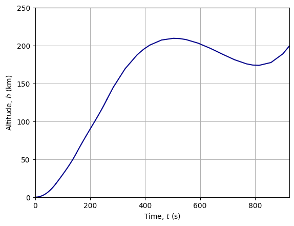
Altitude
[11]:
plt.figure(1)
plt.clf()
for phase in range(4):
    h = np.sqrt(sum(x[phase][i] ** 2 for i in range(3))) - R_e
    plt.plot(t[phase], h / 1000, color[0])
plt.xlim(0, tf)
plt.ylim([0, 250])
plt.xlabel(r"Time, $t$ (s)")
plt.ylabel(r"Altitude, $h$ (km)")
plt.grid("both")
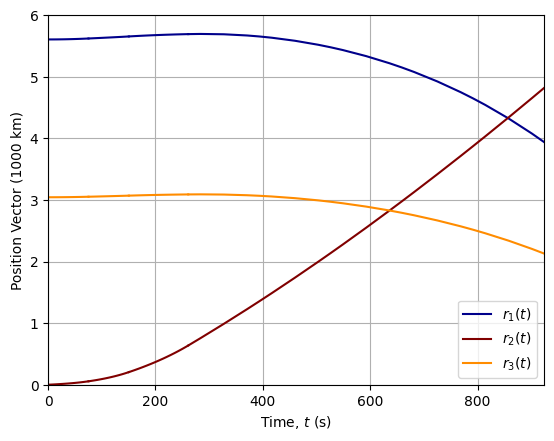
Vehicle Position
[12]:
plt.figure()
for phase in range(4):
    for i in range(3):
        plt.plot(t[phase], x[phase][i] / 1e6, color[i])
plt.legend([r"$r_{1}(t)$", r"$r_{2}(t)$", r"$r_{3}(t)$"])
plt.xlim(0, tf)
plt.ylim(0, 6)
plt.xlabel("Time, $t$ (s)")
plt.ylabel("Position Vector (1000 km)")
plt.grid("on")
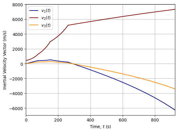
Vehicle Velocity
[13]:
plt.figure()
for phase in range(4):
    for i in range(3, 6):
        plt.plot(t[phase], x[phase][i], color[i - 3])
plt.legend([r"$v_{1}(t)$", r"$v_{2}(t)$", r"$v_{3}(t)$"])
plt.xlim(0, tf)
plt.xlabel("Time, $t$ (s)")
plt.ylabel("Inertial Velocity Vector (m/s)")
plt.grid("on")
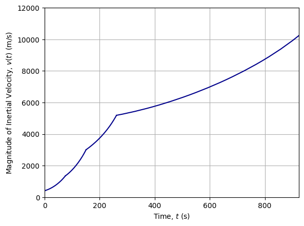
[14]:
plt.figure()
for phase in range(4):
    plt.plot(t[phase], v[phase], color[0])
plt.xlim(0, tf)
plt.ylim([0, 12000])
plt.xlabel("Time, $t$ (s)")
plt.ylabel("Magnitude of Inertial Velocity, $v(t)$ (m/s)")
plt.grid("on")
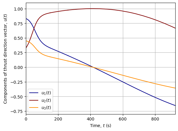
Control Inputs (Thrust Directions)
[15]:
plt.figure()
for p in range(4):
    for i in range(3):
        plt.plot(tc[p], u[p][i], color[i])
plt.legend([r"$u_{1}(t)$", r"$u_{2}(t)$", r"$u_{3}(t)$"])
plt.xlim(0, tf)
plt.ylim([-0.8, 1.1])
plt.xlabel("Time, $t$ (s)")
plt.ylabel("Components of thrust direction vector, $u(t)$")
plt.grid("on")
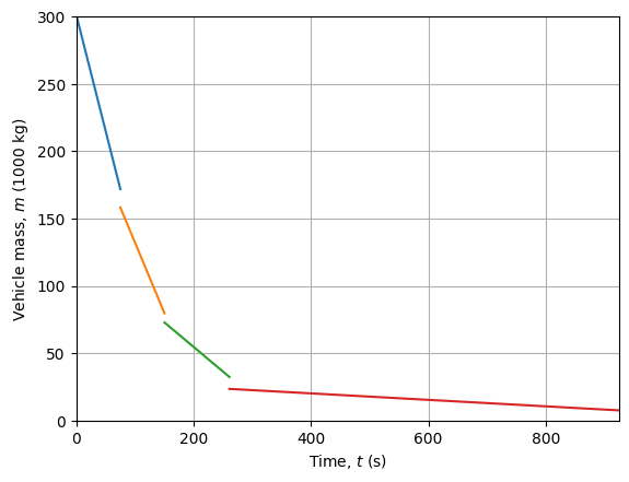
Vehicle Mass
[16]:
plt.figure()
for p in range(4):
    plt.plot(t[p], x[p][6] / 1000)
plt.ylabel("Vehicle mass, $m$ (1000 kg)")
plt.xlim(0, tf)
plt.ylim([0, 300])
plt.xlabel("Time, $t$ (s)")
plt.grid("on")
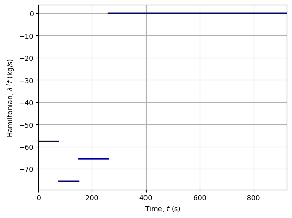
Hamiltonian
The dynamics are time-invariant within phases, and the cost function has no integral terms, and so the Hamiltonian should be be constant within each phase.
[17]:
plt.figure()
for p in range(4):
    plt.plot(tc[p], hamiltonian[p], color[0], linewidth=2)
plt.xlim(0, tf)
plt.xlabel(r"Time, $t$ (s)")
plt.ylabel(r"Hamiltonian, $\lambda^T f$ (kg/s)")
plt.grid("both")