Brachistochrone

For a solution to the brachistochrone problem using a Python script instead of a notebook, see the brachistochrone Python script documentation.

Problem Description

The brachistochrone problem is a classic problem in the calculus of variations. The problem was posed by Johann Bernoulli in June 1696 [1] in a challenge to the mathematicians of his time. The problem can be stated as follows: Given two points A and B in a vertical plane, what is the path that a particle, starting from rest and accelerated by a uniform gravitational force, will take to descend from A to B in the least time? The optimal path, known as a brachistochrone, has the shape of an inverted cycloid.

Formulated as an optimal control problem, the objective of the control problem is to minimize the objective

\[J = t_F\]

where \(t_F\) is the time it takes the particle to move along the curve.

The system has three states: the horizontal position of the particle, \(x\), with the positive direction to the right; the vertical position of the bead, \(y\), with the positive direction down; and the velocity of the particle, \(v\). There is a single control input, \(u\) which is the angle between the velocity vector and the \(x\) axis, so that positive \(u\) corresponds to a velocity vector that points below horizontal.

The equations of motion for the system are

\[\begin{split}\begin{align} \dot x(t) &= v(t) \cos u(t) \\ \dot y(t) &= v(t) \sin u(t) \\ \dot v(t) &= g \sin u(t) \end{align}\end{split}\]

where \(g\) is the acceleration due to gravity.

For this example, we will set the boundary conditions and constraints to be

\[\begin{split}\begin{gather} t_0 = 0 \\ x(t_0) = y(t_0) = v(t_0) = 0 \\ x(t_f) = 1 \\ -\frac{\pi}{2} \le u(t) \le \frac{\pi}{2} \end{gather}\end{split}\]

YAPSS Solution

Import needed modules:

# third party imports
import matplotlib.pyplot as plt

# package imports
from yapss import Problem
from yapss.math import cos, pi, sin

Instantiate the problem and define the callback functions:

# instantiate problem
problem = Problem(name="Brachistochrone", nx=[3], nu=[1])

# gravity constant
g0 = 32.174

# callback functions


def objective(arg) -> None:
    arg.objective = arg.phase[0].final_time


def continuous(arg) -> None:
    # extract the state and control vectors
    x, y, v = arg.phase[0].state
    (u,) = arg.phase[0].control

    arg.phase[0].dynamics[:] = v * cos(u), v * sin(u), g0 * sin(u)


problem.functions.objective = objective
problem.functions.continuous = continuous

Define the bounds on the decision variables:

# problem bounds
bounds = problem.bounds.phase[0]
bounds.initial_time.lower = bounds.initial_time.upper = 0
bounds.final_time.lower = 0
bounds.initial_state.lower[:] = bounds.initial_state.upper[:] = 0
bounds.final_state.lower[0] = bounds.final_state.upper[0] = 1
bounds.state.lower[:] = 0
bounds.control.lower[:] = -pi / 2
bounds.control.upper[:] = pi / 2

Define the initial guess:

# initial guess
phase = problem.guess.phase[0]
phase.time = [0.0, 1.0]
phase.state = [[0.0, 1.0], [0.0, 1.0], [0.0, 1.0]]
phase.control = [[0.0, 0.0]]

Define the computational mesh:

# mesh
m, n = 20, 10
problem.mesh.phase[0].collocation_points = m * [n]
problem.mesh.phase[0].fraction = m * [1 / m]

YAPSS options:

# yapss options
problem.derivatives.method = "auto"
problem.derivatives.order = "second"
problem.spectral_method = "lgr"

Ipopt options:

# ipopt options
problem.ipopt_options.print_level = 3
problem.ipopt_options.print_user_options = "no"
problem.ipopt_options.tol = 1e-20

Find the solution:

# solution
solution = problem.solve()

******************************************************************************
This program contains Ipopt, a library for large-scale nonlinear optimization.
 Ipopt is released as open source code under the Eclipse Public License (EPL).
         For more information visit https://github.com/coin-or/Ipopt
******************************************************************************

Total number of variables............................:      800
                     variables with only lower bounds:      600
                variables with lower and upper bounds:      200
                     variables with only upper bounds:        0
Total number of equality constraints.................:      600
Total number of inequality constraints...............:       61
        inequality constraints with only lower bounds:        1
   inequality constraints with lower and upper bounds:        0
        inequality constraints with only upper bounds:        0


Number of Iterations....: 37

                                   (scaled)                 (unscaled)
Objective...............:   3.1248013070866432e-01    3.1248013070866432e-01
Dual infeasibility......:   3.3305090637068664e-16    3.3305090637068664e-16
Constraint violation....:   1.1053380433168059e-12    1.1053380433168059e-12
Variable bound violation:   0.0000000000000000e+00    0.0000000000000000e+00
Complementarity.........:   2.0021891592803755e-19    2.0021891592803755e-19
Overall NLP error.......:   1.1053380433168059e-12    1.1053380433168059e-12


Number of objective function evaluations             = 38
Number of objective gradient evaluations             = 38
Number of equality constraint evaluations            = 38
Number of inequality constraint evaluations          = 38
Number of equality constraint Jacobian evaluations   = 38
Number of inequality constraint Jacobian evaluations = 38
Number of Lagrangian Hessian evaluations             = 37
Total seconds in IPOPT (w/o function evaluations)    =      0.347
Total seconds in NLP function evaluations            =      0.113

EXIT: Solved To Acceptable Level.

Plots

To plot the solution, we extract the state, control, and costate vector arrays; the time array for the interpolation points (time) and the time array for the collocation points (time_c); the initial and final times; and the dynamics array. Note that the state is defined at the interpolation points (which includes all the collocation points), while the control, costate, and dynamics are defined at the collocation points (which does not include the final interpolation point when using LGR interpolation).

# extract solution
state = solution.phase[0].state
control = solution.phase[0].control
costate = solution.phase[0].costate

time = solution.phase[0].time
time_c = solution.phase[0].time_c
t0 = solution.phase[0].initial_time
tf = solution.phase[0].final_time

f = solution.phase[0].dynamics

x, y, v = state

With the data extracted, we can then plot the results.

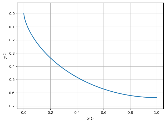
Path of the Bead

# plot bead path
plt.figure()
plt.plot(x, y, linewidth=2)
plt.xlabel("$x(t)$")
plt.ylabel("$y(t)$")
plt.xlim([0.0, 1.0])
plt.ylim([0.7, 0.0])
plt.axis("equal")
plt.tight_layout()
plt.grid()

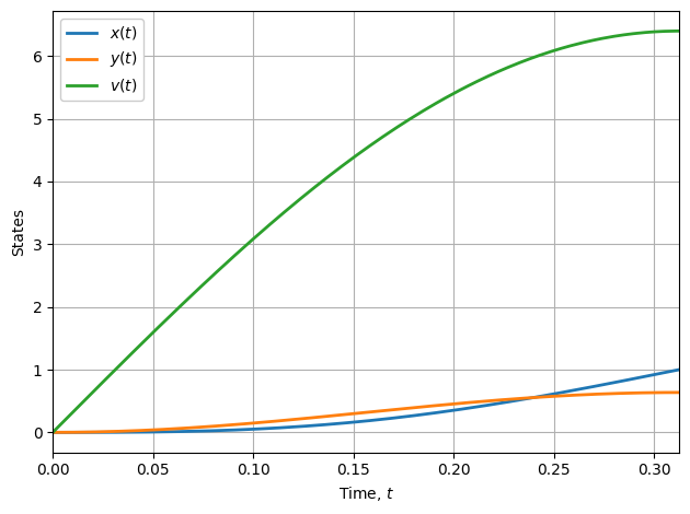
State Trajectories

# plot states vs. time
plt.figure()
plt.plot(time, x, time, y, time, v, linewidth=2)
plt.xlabel("Time, $t$")
plt.ylabel("States")
plt.legend(("$x(t)$", "$y(t)$", "$v(t)$"), framealpha=1.0)
plt.xlim([t0, tf])
plt.tight_layout()
plt.grid()

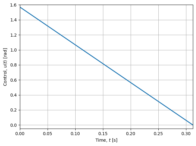
Control History

# plot control vs. time
plt.figure()
plt.plot(time_c, control[0], linewidth=2)
plt.xlabel("Time, $t$ [s]")
plt.ylabel("Control, $u(t)$ [rad]")
plt.ylim([-0.05, 1.6])
plt.xlim([t0, tf])
plt.tight_layout()
plt.grid()

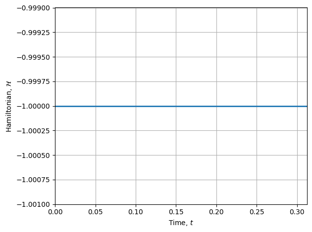
Hamiltonian

Because the dynamics are time-invariant and there is no integral term in the cost function, we expect the Hamiltonian to be a constant. Because the problem is a minimum time problem, we expect that the final value of the Hamiltonian (and hence the value over the entire interval) will be 1. Plotting the Hamiltonian confirms that this is the case:

# plot the Hamiltonian
hamiltonian = sum(f[i] * costate[i] for i in range(3))
plt.figure()
plt.plot(time_c, hamiltonian, linewidth=2)
plt.xlim([t0, tf])
plt.ylim([-1.001, -0.999])
plt.xlabel("Time, $t$")
plt.ylabel(r"Hamiltonian, $\mathcal{H}$")
plt.tight_layout()
plt.grid()

References

[1]

Johann Bernoulli. Problema novum ad cujus solutionem Mathematici invitantur [A new problem to whose solution mathematicians are invited]. Acta Eruditorum, June 1696.